Click on a Lab in the table of Contents then look below for lab descriptions...

Experiment Two: Summation of Forces in Two Dimensions

Newton's First Law of Motion is a description of the inertial property of matter. The law states that an object at rest, or one moving with constant velocity, will remain at rest, or continue with the same velocity, unless acted upon by an external force.

Notice that the law as stated says nothing about how the object came to rest, or acquired its constant velocity. Also notice that that the law does not say that there are no forces acting on an object at rest. An object at rest may have many forces acting on it, but the forces must be acting in such a way that they cancel each other out, leaving a net force of zero.

Newton's First Law does not really say what a force is, only what effect a force has. Interpreted this way, the First Law defines one property of force -- it causes an object at rest to move. It is sufficient to consider a force as a push or a pull.

In this lab you will examine the static equilibrium of a metal ring attached to which are several strings. The strings are arranged as shown in the diagram below, with small weights attached to the end of each string. The pulleys are there only to re-direct the path of the string. You may assume that the pulleys do not affect the metal ring in any way (but is this a good assumption?)

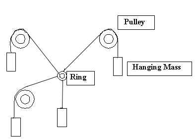
The force of gravity acts on the hanging weights; this force acts to pull the weights downward, but the strings transfer this pull to the metal ring. If the strings and weights are arranged properly, the metal ring will be pulled in several opposing directions and it will remain stationary, even though several forces are acting on it. The ring will be in static equilibrium. Your task is to find out if the forces really do add up to give a zero net force acting on the ring, in accordance with the first condition of equilibrium.
 
 
 

Experiment Three: Summation of Torques in Two Dimensions
 
 

A torque tends to overcome an object's resistance to being rotated (its angular inertia, or Moment of Inertia) and causes an object to spin faster and faster (i.e. gives it an angular acceleration.)

The Second Condition of Equilibrium states that an object which has zero angular acceleration has zero net torque acting on it.

This does not say that an object which is not accelerating about some axis has no torques acting on it - there may be many, but they must be acting so as to cancel each other out. Torques are vector quantities, and so the rules of vector addition apply.

Torques are calculated from the forces acting on the object, and from the positions the forces act with respect to some pivot point, or axis. The magnitude of the torque is equal to the force magnitude times the perpendicular distance from the axis to where the force acts. The direction of the torque is such that it is at right angles to both the force and a line connecting the axis to the force direction. Counter-clockwise rotations are associated with positive torques. Use the Right Hand Rule to figure out the torque direction. Curl the fingers of your right hand in the direction of rotation of the object. Your thumb will point in the direction of the torque.

The apparatus consists of a ball resting on a nearly frictionless air bearing. Attached to the ball are six metal rods. Attached to the end of each rod is a string with a mass hanger. You are to put masses on the hangers so that the ball remains in static equilibrium, then calculate the torques acting based on your measurements of the forces, and their perpendicular distances from the pivot axis. The apparatus has been designed to make these measurements fairly easy to obtain. Read through the procedure section of the manual carefully before proceeding.

Having calculated the torques, you will try to show that their vector sum is zero, in accordance with the Second Condition of Equilibrium.
 

Experiment Four: Constant Velocity in One Dimension

The inertial properties of a mass determine how it acts under the influence of a force. Newton's First Law states that an object at rest, or moving with constant velocity, will remain at rest, or continue with the same constant velocity unless acted upon by an external force. The major difficulty in investigating this is the removal of external forces. Gravity is present in the lab, and despite our best efforts, we've been unable to convince granting agencies to fund our programme of anti-gravity research. Similarly, friction is always present, and is one of the main reasons it took so long for people to come to an understanding of simple motion.

To overcome the effects of the forces of gravity and friction, you will use an air track. With this device, a small cart rides on a cushion of air along a horizontal track. By giving the cart a gentle push to start it, you can examine the motion of the cart as it travels along the track, and you can assume that no force will disturb its motion.

You will measure the position, velocity, and acceleration of the cart and perform some statistical analysis of the measurements. You will try to verify Newton's first law by showing that the cart does not accelerate in the absence of a net force.
 

Experiment 7: Conservation of Momentum in One Dimension

Momentum is defined as mass times velocity, so can be considered as a measure of the 'amount of motion' of an object.

For a system consisting of two or more objects which are interacting with one another, the total momentum of the system is a constant. For example, if two objects collide, the momenta of the two objects before the collision occurs is equal to the momenta of the two after the collision.

In this lab you will study the collision of two carts on an air track. The collision will be perfectly inelastic, that is, the two carts will stick together after the collision. You will measure the mass and velocity of each cart, then calculate their momenta before and after the collision to check if the total momentum really is conserved. You will also check to see if the Kinetic Energy is conserved. (Do you predict that it will, or won't be conserved?)
 

Experiment 9II: Conservation of Momentum in Two Dimensions

Conservation of Momentum is a fundamental principle in physics. If momentum is considered as a measure of the amount of motion in a system of interacting objects, then the conservation principle simply states that the amount of motion in the system does not change as the objects interact, no matter what the form of the interaction.

Linear Momentum is defined as mass times velocity, and since velocity is a vector, linear momentum must also be a vector.

In this lab you will use an Air Table to examine the collision of two pucks. The pucks ride on a thin layer of air, and can be considered nearly frictionless. The pucks are fitted with magnets of like polarity so that they repel each other. The collision, then, is a magnetic one - it is very important that the pucks make no physical contact with one another.

You will measure the position and velocity of each puck before and after the collision occurs. Using this data you will be able to determine the momentum of each puck before and after the collision. Using the rules for vector addition in two-dimensions, you will then be able to calculate the total momentum of the system consisting of the two pucks before and after the collision. You can then compare these momenta to see if the total momentum remained a constant, in accordance with the conservation principle described above.

You will also check to see if Kinetic Energy is conserved in the system. The Kinetic Energy of an object is defined as:
 
 

K.E. = (mv²)/2

m is the mass of the object in kilograms (kg)

v is the velocity of the object in metres/second (m/s)

If the Kinetic Energy is conserved, then the collision is said to be perfectly elastic.
 

Experiment 8: Acceleration in One Dimension

A force applied to an object will cause the object to accelerate. The inertia of the object, a property defined by the mass, provides a resistance to the force, and so restricts the amount of the acceleration the force can cause. The relation between force, mass, and acceleration is summarised in Newton's Second Law of Motion:

F = ma

F is the net force, in Newtons (N)

m is the mass, in kilograms (kg)

a is the acceleration, in metres/second/second (m/s2)

The acceleration will be along the direction defined by the applied force.

Notice that the force referred to here is really the net force acting. An object may experience many forces, but the resulting acceleration will be defined by the vector sum resultant of all the forces acting.

In this lab you will investigate the motion of a cart on an Air Track as several forces act on the cart. The net force will be supplied by a small mass hanging on the end of a string. The string will pass over a pulley to redirect the force from the vertical to the horizontal. The other end of the string will be attached to the cart.

You will measure the position, velocity, and acceleration of the cart, and the total mass of the accelerated system. (What exactly is being accelerated?) You will also calculate the net force acting on the cart based on the mass of the hanging weight and the gravitational force of attraction between the Earth and the hanging weight. Using this data, you will then try to verify the Second Law of Motion.
 

Experiment 9I: The Acceleration Due to Gravity

In 1687, Newton published a Theory of Universal Gravitation which states that every mass attracts every other mass with a force proportional to the mass of each, and inversely proportional to the square of the distance between their centres. Symbolically this is written:
 
 

F = GMm/R²

F is the gravitational force in Newtons (N)

M is the mass of one object in kilograms (kg)

m is the mass of another object

R is the centre to centre separation of the objects in metres (m)

G is a constant 6.67 x 10 ^-11 Nm²/kg²

Notice that this expression defines the interaction force between two masses. Each mass applies the same force to the other. The force is attractive, and is directed along the line joining the centres of the objects.

According to the Second Law of Motion, an applied force causes an acceleration. So, two masses should accelerate toward each other due to the gravitational force described above. In particular, a mass near the surface of the Earth should be accelerated toward the centre of the Earth.

In this lab, you will try to measure this acceleration.

You will use an Air Table on which rides a small puck supported by a thin layer of air. As you may have noticed, objects fall rapidly when dropped, presenting some difficulties for anyone trying to measure the position, velocity, and acceleration of a falling object. You will overcome this problem easily by providing a less vertical path for the falling puck by slightly tipping the Air Table from the horizontal. With this method, you will be able to measure the position, velocity, and acceleration of the puck. You will then compare the measured acceleration with that predicted by the Universal Theory equation above. Write down the expression for the acceleration.
 
 
 

Experiment 12: Hooke’s Law

In the mid-17th century, Robert Hooke showed that if a force is applied to a solid, the resulting deformation is proportional to the applied force. This relation only holds over the range of forces sufficient to cause small deformations. Nevertheless, the relation holds over a wide range of materials, and has many important applications in engineering, materials science, and structural bio-materials engineering.

The relation, now known as Hooke's Law, applies particularly well to helical springs. A helical spring is a piece of wire wound around in the form of a helix. If a weight is attached to one end, while the other end is held fixed, the spring will stretch. According to Hooke's Law, the amount of stretch will be directly proportional to the amount of weight on the spring. This can be written as:
 
 

F = -kx

F is the restoring force, in Newtons

x is the amount of stretch in metres

k is the spring constant of proportionality

The spring constant is a measure of the stiffness of the spring - it describes how much force is required to stretch or compress the spring a given distance.

Notice the minus sign in the equation. The Force represented by F is the restoring force of the spring. It acts to restore the spring to its equilibrium position (which is usually the unstretched position.)

Adding a weight to the spring causes it to be stretched downward until the mass reaches an equilibrium position. The force of gravity acts downward on the hanging mass. According to Newton's Third Law, though, an equal, opposite force must act upward on the mass, if it is in equilibrium. This upward force is supplied by the spring, and is the restoring force. Notice that the minus sign is required so that the upward restoring force in this case, is opposite to the downward stretch of the spring.

In this lab you will try to verify Hooke's Law for a helical spring by measuring the stretch of the spring as you add weight to it.
 

Experiment 10: Conservation of Angular Momentum

Angular Momentum is a quantity which can be considered as measuring the "amount of rotation" an object has. For a system consisting of many interacting objects, the total angular momentum is a constant. This is known as the fundamental principle of the Conservation of Angular Momentum.

Angular Momentum is defined as:
 
 

L = Iw

I is the Moment of Inertia in kgm²

w is angular velocity in radian/s

The Moment of Inertia of an object is a measure of the inertia the object has with respect to an acceleration about some axis. It is a measure of the resistance an object presents to being rotated under the action of a torque. Under this description, the Moment of Inertia depends upon the mass of an object, and the distribution of that mass about the axis of rotation.

A single object has as many Moments of Inertia as it has possible axes of rotation.

In this lab you will measure the angular velocities of two plastic platters. The platters will be rotating about an axis through their centres and perpendicular to the plane of the platters, just like an old style record player ... the kind your parents may have used long, long ago as they huddled by the fire in their cold, damp cave.

You will cause the platters to collide by dropping one onto the other. In this collision, the platters will acquire the same speed after the collision, and will be effectively stuck together. The collision will therefore be perfectly inelastic.

Due to the symmetry of the platters about the rotation axis, the Moments of Inertia are fairly easy to calculate (you will be shown how to do this.) You will measure the velocities, so you will be able to calculate the angular momentum of each platter before and after the collision. You will then be able to determine if the total angular momentum has been conserved, in accordance with the principle stated above.
 

Experiment 11: Moments of Inertia

The Moment of Inertia of an object is a measure of the inertia the object has with respect to an acceleration about some axis. It is a measure of the resistance an object presents to being rotated under the action of a torque. Under this description, the Moment of Inertia depends upon the mass of an object, and the distribution of that mass about the axis of rotation.

A single object has as many Moments of Inertia as it has possible axes of rotation.

In this lab you will try to figure out the Moment of Inertia of a flywheel. The flywheel is actually a combination of objects of different shapes and masses. These objects will be constrained so that they can rotate only about an axis through their centres. Believe it or not, this really does simplify your task.

You will measure the acceleration of the flywheel as it rotates under the action of a torque. From this, and measurements of the mass and mass distribution of the flywheel's components, you should be able to calculate the Moment of Inertia (honestly.) You should also be able to predict the Moments of each component of the flywheel based on their symmetry with respect to the axis of rotation (you'll be shown how), then compare your predicted value against your calculated value. The two will agree reasonably well. They really will. Really.

No kidding.
 

Experiment 13: Standing Waves on a String

If a string is held fixed at one end, and oscillated at the other, waves will travel along the string from one end to the other, and back again. The waves are called transverse because the wave motion (the string wiggling up and down) is at right angles to the direction of motion of the wave along the length of the string. The waves are reflected at each end of the string, and the reflected waves travel back the way they came, but upside down. The reflected waves are 180 degrees out of phase.

The principle of Superposition states that waves can be added together. Adding two waves that are 180 degrees out of phase results in a complete cancellation. It would seem that, at least for some of the time, the string will be completely flat. The waves, though, are travelling waves, so the flat-line condition will not be permanent. At another time, the waves will combine to produce a "super" wave with maximum crests and troughs.

The particular form that the string adopts depends on the frequency of the oscillation supplied at one end, the tension in the string, and the density of the string. For particular values of these, standing waves can be set up in the string. The standing wave pattern is characterised by the fact that all portions of the string undergo simple harmonic motion with an amplitude which depends on the position along the string. Some places on the string will not oscillate at all - the amplitude is zero. These are called nodes. Other positions will undergo maximum oscillations - the amplitude is a maximum. These are called antinodes. The wave is called "standing" because the nodes and antinodes do not travel along the string.

Standing waves are not restricted to strings. The laser (Light Amplification through the Stimulated Emission of Radiation) is an example of a standing wave in light. Standing waves can also be used to describe some quantum-mechanical effects relating to the behaviour of matter at the atomic scale.

In this lab you will set up standing waves on a string. The string will be oscillated at one end with a fixed frequency. You will adjust the tension in the string to set up various standing waves. You will then measure the wavelength of the travelling waves which form the standing wave pattern, then calculate the velocity of the travelling waves using the relation:
 
 

v² = T/(ml²)

v is the wave velocity in metres/second

T is the string tension in Newtons
 
 

l is the wavelength in metres
 
 

m is the string density in kilograms/metre

You will then calculate the frequency of the oscillator based on the velocity calculated above, and the following relation between frequency, wavelength, and velocity:

v = ln

n is the wave frequency in Hertz, or 1/second

Finally, you will compare the calculated frequency against the measured frequency of the oscillator.
 

Experiment 17I: Converting a Galvanometer

An object with an electric charge moving in a magnetic field is subject to a force. This is a fact, and an example of the profound relation between electricity and magnetism. The force is at right angles to the direction of motion of the charged object, and to the direction of the magnetic field lines. The Right Hand Rule is helpful in determining the direction of the force.

This interaction between charges and magnetic fields can be exploited to make mass spectrometers, motors, generators, and simple electrical meters. In this lab you will convert a galvanometer into a voltmeter and an ammeter.

A D'Arsonval galvanometer consists of a finely wound coil of wire suspended in the magnetic field of a permanent magnet. The coil is free to rotate about an axis at right angles to the magnetic field lines.

When an electric current flows through the wire, the charges comprising the current are forced to move at right angles due to the presence of the magnetic field. The charges, though, cannot leave the wire. The wire, though, can rotate, which it does. The amount it rotates is proportional to the amount of moving charge present, in other words to the amount of current.

Attached to the coil is a pointer. The position of the pointer is read off against a scale.

The galvanometer, then, is a device for measuring current. Most galvanometers are very sensitive and delicate and must be handled with care (something like the university administrators.) They are far too delicate, in fact, to be used regularly in a laboratory setting for making routine measurements (much more like your professors.) To make a more robust instrument, you will modify the galvanometer to make it capable of measuring a wider range of current.

This is done in a straightforward way (if you know how). What you really need to do is to figure out a way to restrict the current flowing into the galvanometer without restricting the current flowing elsewhere in the circuit in which you are making the measurement.

When was the last time you rode on the railway? Probably a long time, but the railway is not a bad analogy. Think about the electrical circuit as some arrangement of rails. The current is the train. If you want to measure the flow of train cars past a certain point, you might put some device on the track to do that. That's your galvanometer. But, if the whole train runs over it, it will be ruined. At best, it can handle being hit with one car. What you need to do is set up the galvanometer so that only one car out of every 100 cars goes through the galvanometer, then you just take the reading, and multiply by 100.

But how do you pick out only one car? When you want to make a measurement, place a small run of rail line parallel to the galvanometer, then put the galvanometer on the main line. All you need to do is make sure that one car goes through the galvanometer, and the rest go through the parallel bit of track. That way, all the cars stay on the main track, so the total number of cars hasn't changed. The small run of parallel track is called a shunt line.

Of course, electrical circuits aren't railway lines, and currents aren't trains, but the basic principle of the shunt is exactly the same in both cases. In a typical circuit, the current flowing is much too large to be measured by a galvanometer. So, you must add a shunt - a small resistor - to redirect a small portion of the current through the coil in the galvanometer, while most of the current goes through the shunt. The details of how to calculate the value of the shunts, and how to connect the galvanometer into a circuit are found in the lab manual.
 

Experiment 22b: The Coulomb Balance

Electrical charge comes in two types, designated positive and negative. Unlike charges attract one another with a force proportional to the charges, and inversely proportional to the square of the distance between them. The nature of this force is clearly demonstrated by the device called the Coulomb Balance.

The Coulomb Balance consists of two parallel metal plates. The bottom plate is held fixed; the top one is balanced above it. The two plates are not electrically connected. If you were to generate a large potential difference across the plates using a power supply, you would find that the top plate would move toward the bottom one. If you assume that one plate becomes negatively charged with respect to the other, then the movement of the top plate can be explained as being due to the Coulomb force of attraction between the plates. Your task is to determine the magnitude of that force.

If the plates are parallel when the force is acting, then the Balance can be treated as a parallel plate capacitor. The relation describing the force in such a device is:
 
 

F = e₀AV²/2d²

F is the electrical force of attraction in Newtons

A is the cross sectional area of the plates in metres squared

V is the potential difference across the plates in Volts

d is the separation between the plates in metres
 
 

e₀ is the permittivity constant in Farads/metre

To determine the electrical force acting, you will first apply a known weight sufficient to bring the top plate down to a specific position. You will remove the weight, then apply a sufficient potential difference to cause the top plate to move down to the same position. This will allow you to equate the known gravitational force to the electrical force.

Once you know the force (F in the equation) you can then solve for the remaining unknown, e₀ (epsilon nought). This constant is called the permittivity of free space.

In the 1880s Maxwell unified the then quite separate phenomenon exhibited by electrified matter and magnetised matter. He showed that each was related to the other by deducing a set of four equations which beautifully described all known electromagnetic phenomena. This was an outstanding achievement which even led some scientists of the day to claim that Physics had come to an end, since all was now known. Not only did Maxwell's equations describe all things electromagnetic, they even permitted him to predict the existence of electromagnetic waves, and their speed of propagation. In the equations appear two fundamental constants, the permittivity and permeability of free space. You will use your data from this lab to calculate the permittivity constant, and then the propagation speed of electromagnetic waves, then compare these against the standard values.
 

Experiment 17II: Series and Parallel Direct Current Circuits

In this lab you will construct simple direct current circuits using several resistors in series and parallel combinations. You will then measure currents and potential differences in order to verify Ohm's law for multiple resistor circuits.
 

Experiment 14: Sound Waves in Air

Sound waves consist of a series of compressions (density increases) and rarefactions (density decreases) of the air. The wave action (the air molecules locally oscillating back and forth) is in the same direction as the wave motion, hence the sound wave is called longitudinal.

If a sound wave is generated at one end of a column of air, the other end of which is closed, the wave will propagate to the closed end, then be reflected back up the column. The reflected wave will be inverted with respect to the original wave; it will be 180 degrees out of phase.

The principle of Superposition states that waves can be added together. Adding two waves that are 180 degrees out of phase results in a complete cancellation. It would seem that, at least for some of the time, the air would be neither compressed nor rarefied. This would suggest that there would be no sound coming from the tube. The waves, though, are travelling waves, so the no-sound condition will not be permanent. At another time, the waves will combine to produce a "super" wave with maximum sound loudness.

The particular form that the air in the column adopts depends on the frequency of the oscillation supplied at one end and the density of the air. For particular values of these, standing waves can be set up in the column. The standing wave pattern is characterised by the fact that all the air in the column undergoes simple harmonic motion with an amplitude which depends on the position along the column. Some places in the column will not oscillate at all - the amplitude is zero. These are called nodes. Other positions will undergo maximum oscillations - the amplitude is a maximum. These are called antinodes. The wave is called "standing" because the nodes and antinodes do not travel along the column.

Standing waves are not restricted to air columns. The laser (Light Amplification through the Stimulated Emission of Radiation) is an example of a standing wave in light. Standing waves can also be used to describe some quantum-mechanical effects relating to the behaviour of matter at the atomic scale.

In this lab you will set up standing waves in an air column. The air will be oscillated at one end with a frequency fed into an audio speaker. You will adjust the frequency to set up various standing waves. You will then measure the wavelength of the travelling waves which form the standing wave pattern, then calculate the velocity of the travelling waves using the relation:
 
 
 
 

v = ln

v is the velocity of the travelling waves in metres/second
 
 

l is the wavelength in metres
 
 

n is the wave frequency in Hertz, or 1/seconds

You will then calculate the velocity of the wave based on the air temperature (you will be shown how.) What you will have calculated is more familiarly known as the speed of sound (in air.) Finally, you will compare the calculated speed against the measured speed.
 

Experiment 22a: The Current Balance

A moving charge is a source of a magnetic field. If another charge is moving nearby, then its magnetic field will interact with the magnetic field produced by the other moving charge. This interaction is clearly demonstrated by a device called a Current Balance.

The Current Balance consists of two parallel wires. The bottom wire is fixed; the top one is balanced above it. The two wires are electrically connected in series. When current passes through the bottom wire in one direction, the same current passes through the top conductor in the opposite direction. The currents generate magnetic fields since the currents are moving charges. Will the magnetic fields cause the top conductor to be attracted to, or repelled by the bottom one?

The only way to answer this is to figure out the direction of the magnetic fields generated by a moving charge. This can be done analytically (see your textbook, or class notes) or you can use the Right-Hand Rule: Imagine that you grasp the wire in your right hand, with your thumb pointing in the direction of the current flow. Your fingers will then curl around in the direction of the magnetic field lines. Be advised that it is never a good idea to grasp any wires, especially when you know they are carrying a current. You are only supposed to pretend to grasp the wire.

If you apply this method to two parallel wires carrying anti-parallel currents, you will discover that the direction of the magnetic field lines due to each conductor in the space between the wires are in the same direction. Since the same polarity magnetic fields repel, it would seem that you can predict that the wires in the Current Balance will repel one another.

You will measure the repelling force between the conductors by measuring how much current is required to separate the conductors by a specific distance, while loading the top conductor with a series of weights. This will give you a set of data comprised of currents and forces. You will then determine the relation between these two parameters, and compare your conclusion against the theoretically predicted relation.

In the 1880s Maxwell unified the then quite separate phenomenon exhibited by electrified matter and magnetised matter. He showed that each was related to the other by deducing a set of four equations which beautifully described all known electromagnetic phenomena. This was an outstanding achievement which even led some scientists of the day to claim that Physics had come to an end, since all was now known. Not only did Maxwell's equations describe all things electromagnetic, they even permitted him to predict the existence of electromagnetic waves, and their speed of propagation. In the equations appear two fundamental constants, the permittivity and permeability of free space. You will use your data from this lab to calculate the permeability constant, and then the propagation speed of electromagnetic waves, then compare these against the standard values.

The Current Balance is used in practise to define the standard value of the Ampere, the unit of current.
 

Experiment 18: RC Circuit

A capacitor is a device used for storing electrical charge.  In a direct current circuit it is used with a resistor to control the rate of current flow in the circuit.  The RC circuit, then, is a simple timing circuit.  Turn signal indicators in cars, variable windshield wiper control, flash discharge control for photographic cameras, and timing control for battery rechargers are some examples of the common uses of simple RC circuits.

In this lab you will construct a simple RC circuit, charge a capacitor, then measure the rate at which the capacitor discharges through a resistor.  From the decay curve, you will determine the time constant for the circuit, then calculate the capacitance of the capacitor to compare against the manufacturer's supplied value.

The time constant is the time it takes for the capacitor to discharge to 36.8 percent of its fully charged value.  The percentage quoted may seem a strange value, but it is actually a reasonable value because it represents the time it takes the capacitor to discharge to 1/e of its fully charged value.  "Oh, that's much better" you say?  Well, yes, for an exponential discharge it is much better.  The potential difference across the capacitor is described by the following exponential function:

V = V₀e^(-t/RC)

V₀ is the initial potential difference in volts
R is the resistance in ohms
C is the capacitance in Farads
t is the time in seconds

So, you can see that when t = RC (the time constant), then V has dropped to V₀e^-1, or 1/e of its original value.  If you calculate 1/e, you will find that it equals .368, and that's why the percentage given above is a reasonable definition for the time constant.
 
 
 
 
 
 
 
 

Experiment 21: Motors and Generators
 
 
 
 

Experiment 15: The Electrical Equivalent of Heat

Heat, once thought to be a substance which flowed from a hotter object to a cooler one, is now considered a form of energy.

If heat is a form of energy, then it should be possible to find an equivalence between it and other forms of energy. In this lab you will calculate the electrical equivalent of heat. You will do this by heating a known quantity of water by supplying it with electrical energy. Based on the temperature increase of the water, you will calculate the increase in energy of the water, then compare this with the electrical energy supplied. In an attempt to prevent heat loss from the water to the surroundings, you will use a simple double-walled calorimeter to contain the water.

The temperature of an object is related to the amount of heat energy contained in the object. The following relation defines the specific heat of a substance in terms of the temperature change of the substance after a quantity of heat energy is transferred to the surroundings:
 
 

Q = mc(DT)

Q is the transferred heat energy in Joules

m is the mass of the substance in kilograms
 
 

DT is the temperature change of the substance in degrees Kelvin

c is the specific heat of the substance in Joules/kg*degrees K

Note that Q and DT are defined to be negative if the substance loses heat.

This relation assumes that the specific heat value is independent of temperature, which it usually is to within a few percent. It also assumes that pressure and volume changes during the heat transfer have no effect on the specific heat. This is approximately true for most solids and liquids, but is not generally correct for gases.

In the experiment, you will use a double-walled calorimeter containing a measured amount of water at a measured temperature.

Immersed in the water are a thermometer, a stirrer, and an electrical heating coil. The coil is connected to a power supply. A current passing through the coil will cause the coil to heat up. By providing a measured current at a measured voltage for a measured time, you can calculate the total electrical energy supplied to the coil:
 
 

E = IVt

I is the current in Amperes

V is the potential difference in Volts

t is the time in seconds

Next, you will calculate the total heat energy transferred from the coil to the calorimeter and its contents. In the calorimeter used, there are several components to consider. The temperature of the water, the inner vessel of the calorimeter, the thermometer, the stirring mechanism, and the heating element will all increase. The specific heats of these materials will be supplied. You will need to calculate the total heat energy gained by these components.

Finally, you will compare the electrical energy supplied to the coil with the heat gained by the components of the calorimeter. They should be exactly the same. Can you suggest any reasons why they may differ?
 

Experiment 19: An Alternating Current RLC Circuit

Alternating Current is the term used to describe a current that varies with time.  The common form of this is a sinusoidally varying current.  In practice, this is supplied by a voltage source that varies sinusoidally.  The voltage source is characterised by a peak voltage, and a frequency.  For example, normal household voltage has a peak voltage of about 170 volts, and a frequency of 60 Hz.  The phase (i.e. when the peaks occur) of the voltage can also be defined.  Generally, the phase of the current in a circuit is shifted with respect to the voltage.

An RLC circuit is a circuit that contains a resistor (R), an inductor (L), and a capacitor (C).
In the circuit you will investigate, you will connect these three components in series.

You will measure the voltage drops across each component, and the phase angle between the source voltage and the total circuit voltage drop. You will be able to calculate the total impedance of the circuit  from the measured voltages. Impedance in an Alternating Current circuit differs from resistance in a Direct Current circuit in that the impedance of non-resistive components such as inductors and capacitors is frequency-dependent.  Phase angle refers to the difference in time between when the peak current through a circuit component occurs compared to when the peak voltage occurs.

You will then calculate the total impedance in the circuit based on the measured source voltage, and you will calculate the phase angle between the source voltage and the total current.

Finally, you will compare the measured impedance and phase angle against the calculated impedance and phase angle.  Think about what might account for any discrepancies.
 
 
 
 
 
 
 

Lab 21