Gini coefficient
From Wikipedia, the free encyclopedia.
The Gini coefficient is a measure of inequality developed by the Italian statistician Corrado Gini and published in his 1912 paper "Variabilità e mutabilità". It is usually used to measure income inequality, but can be used to measure any form of uneven distribution. The Gini coefficient is a number between 0 and 1, where 0 corresponds with perfect equality (where everyone has the same income) and 1 corresponds with perfect inequality (where one person has all the income, and everyone else has zero income). The Gini index is the Gini coefficient expressed in percentage form, and is equal to the Gini coefficient multiplied by 100.
While the Gini coefficient is mostly used to measure income inequality, it can also be used to measure wealth inequality. This use requires that no one has a negative net wealth.
Contents |
Calculation
The small sample variance properties of G are not known, and large sample approximations to the variance of G are poor. In order for G to be an unbiased estimate of the true population value, it should be multiplied by n/(n-1).
The Gini coefficient is calculated as a ratio of the areas on the Lorenz curve diagram. If the area between the line of perfect equality and Lorenz curve is A, and the area underneath the Lorenz curve is B, then the Gini coefficient is A/(A+B). This ratio is expressed as a percentage or as the numerical equivalent of that percentage, which is always a number between 0 and 1.

The Gini coefficient is often calculated with the more practical Brown Formula shown below:
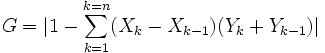
G: Gini coefficient
X: cumulated proportion of the population
variable
Y: cumulated proportion of the income variable
Advantages of the Gini coefficient as a measure of inequality
- The Gini coefficient's main advantage is that it is a measure of inequality, not a measure of average income or some other variable which is unrepresentative of most of the population, such as gross domestic product.
- Gini coefficients can be used to compare income distributions across different population sectors as well as countries, for example the Gini coefficient for urban areas differs from that of rural areas in many countries (though the United States' urban and rural Gini coefficients are nearly identical).
- The Gini coefficient is sufficiently simple that it can be compared across countries and be easily interpreted. GDP statistics are often criticised as they do not represent changes for the whole population, the Gini coefficient demonstrates how income has changed for poor and rich. If the Gini coefficient is rising as well as GDP, poverty may not be improving for the vast majority of the population.
- The Gini coefficient can be used to indicate how the distribution of income has changed within a country over a period of time, thus it is possible to see if inequality is increasing or decreasing.
- The Gini coefficient satisfies four important principles; Anonymity, it doesn’t matter who the high and low earners are. Scale independence, the Gini coefficient does not consider the size of the economy, the way it is measured, or whether it is a rich or poor country on average. Population independence, it does not matter how large the population of the country is. Transfer principle. This states that if we transfer income from a rich person to a poor person, the resulting distribution is more equal.
Disadvantages of the Gini coefficient as a measure of inequality
- The Gini coefficient measured for a large geographically diverse country will generally result in a much higher coefficient than each of its composing regions has. For this reason the scores calculated for individual countries within the E.U. are difficult to compare with the score of the entire U.S.
- Comparing income distributions among countries may be difficult because benefits systems may be different in different countries. For example, some countries give benefits in the form of money, others use food stamps, which may or may not be counted as income in the Lorenz curve and therefore not taken into account in the Gini coefficient.
- The measure will give different results when applied to individuals instead of households. When different populations are not measured with consistent definitions, comparison is not meaningful.
- The Lorenz curve may understate the actual amount of inequality if the situation is that richer households are able to use income more efficiently than lower income households. From another point of view, however, the measured inequality also may be the result of more or less efficient use of household incomes.
- As for all statistics, when collecting the income data initially, there will always be systematic and random errors. If the data is less accurate, then the Gini coefficient has less meaning. Also, countries may measure the statistics differently, thus it is not always possible to compare statistics between countries.
- Economies with similar incomes and Gini coefficients can still have very different income distributions. This is because the Lorenz curves can have different shapes and yet still yield the same Gini coefficient. As an extreme example, an economy where half the households have no income, and the other half share income equally has a Gini coefficient of ½; but an economy with complete income equality, except for one wealthy household that has half the total income, also has a Gini coefficient of ½.
- It is claimed that the Gini coefficient is more sensitive to the income of the middle classes than to that of the extremes.
- Too often only the Gini coefficient is quoted without describing the proportions of the quantiles used for measurement. As with other inequality coefficients, the Gini coefficient is influenced by the granularity of the measurements. Example: Five 20% quantiles (low granularity) will yield a lower Gini coefficient than twenty 5% quantiles (high granularity).
As one result of this criticism, additionally to or in competition with the Gini coefficient entropy measures are used more frequently (e.g. from Atkinson and Theil). These measures attempt to compare the distribution of resources by intelligent players in the market with a maximum entropy random distribution, which would occur if these players would act like non-intelligent particles in a closed system just following the laws of statistical physics.
Gini coefficients of income in selected countries
Development of Gini coefficients in the US over time
Gini coefficients for the United States at various times, according to the US Census Bureau:
2004 Gini coefficients in selected countries
(from the United Nations Human Development Report 2004).
See complete listing in list of countries by income equality.
Hungary:       0.244
Denmark:       0.247
Japan:         0.249
Sweden:        0.250
Germany:       0.283
India:         0.325
France:        0.327
Canada:        0.331
Australia:     0.352
UK:            0.360
Italy:         0.360
USA:           0.408
Singapore:     0.425
Thailand:      0.432
China:         0.447
Russia:        0.456
Guatemala:     0.483
Malaysia:      0.492
Hong Kong:     0.500
Mexico:        0.546
Chile:         0.571
Congo:         0.613
Namibia:       0.707
It is an interesting fact that while the most developed European nations tend to have income inequality values between 0.24 and 0.36, the United States has been above 0.4 for two decades, showing the United States has a greater inequality (and that this is not just a recent development). This is an approach to quantify the perceived differences in welfare and compensation policies and philosophies. However it should be borne in mind that the Gini coefficient can be misleading when used to make political comparisons between large, geographically and culturally diverse countries like the U.S. and smaller, more homogeneous countries like Denmark.
For example, Hungary and Denmark, the two E.U. member countries listed above with the lowest coefficients, are calculated separately by the United Nations, while New Jersey and Mississippi are calculated together as part of the U.S., despite the fact that New England and the deep South of the U.S. are vastly different economic regions with wide differences in cost of living and average income.
Considered together, Hungary and Denmark have a higher Gini score than the U.S. as does the entire European Union if all member states are lumped together. Conversely, when each state or geographical region in the U.S. is considered separately, the Gini scores will generally be lower than those calculated for the entire country.
References
Dixon, PM, Weiner J., Mitchell-Olds T, Woodley R. Boot-strapping the Gini coefficient of inequality. Ecology 1987;68:1548-1551.
Gini C. "Variabilità e mutabilità" (1912) Reprinted in Memorie di metodologica statistica (Ed. Pizetti E, Salvemini, T). Rome: Libreria Eredi Virgilio Veschi (1955).
See also
- List of countries by income equality
- Welfare economics
- Income inequality metrics
- ROC analysis
- Social welfare (political science)
- Pareto distribution
External links
- Measuring income inequality: a new database, with link to dataset
- UN Human Development Report 2004, p50-53: Gini Index calculated for all countries.
- [1] Comparison of Urban and Rural Areas' Gini Coefficients Within States
- [2] World Income Inequality Database
- [3], Forbes Article, In praise of inequality
- Software:
- Free Online Calculator computes the Gini Coefficient, plots the Lorenz curve, and computes many other measures of concentration for any dataset
- Free Calculator: Online and downloadable scripts (Python and Lua) for Atkinson, Gini, Hoover and Kullback-Leibler inequalities
- Users of the R data analysis software can install the "ineq" package which allows for computation of a variety of inequality indices including Gini, Atkinson, Theil.

