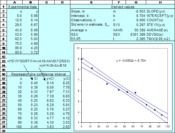
Regression
Analysis - Confidence Interval of the Line of Best Fit
The line of best fit (y = mx + b) is computed from a random sample of measurements of x and y. If we used a different data set we would most likely compute slightly different values for the m and b parameter. Thus our values are always estimates and as such have a confidence interval associated with them.
The confidence interval for the predicted y
value for a given value of the independent variable x is computed
using: 
where t is the critical t statistic,
Syx the standard error of the estimate, xi
the given value of x, ![]() is the average of the
x values and n is the number of observations used in the regression
analysis. As shown in the diagram, we can used various Excel functions
(including TINV, STEYX, DEVSQ ) to compute the confidence interval. The formula
in B18 is =t*SYX*SQRT(1/n+(A18-XAVG)^2/SSX) and in C18 we use =(m*A18+b)+B18.
Note that date in A3:A11 and in B3:B11 is named x and y,
respectively, and that the labels in F2:F8 are used to name the values in
G2:G8. Click here to open the sample
Excel file.
is the average of the
x values and n is the number of observations used in the regression
analysis. As shown in the diagram, we can used various Excel functions
(including TINV, STEYX, DEVSQ ) to compute the confidence interval. The formula
in B18 is =t*SYX*SQRT(1/n+(A18-XAVG)^2/SSX) and in C18 we use =(m*A18+b)+B18.
Note that date in A3:A11 and in B3:B11 is named x and y,
respectively, and that the labels in F2:F8 are used to name the values in
G2:G8. Click here to open the sample
Excel file.
It is important to realise that in this
exercise we are computing the confidence level for the mean response.
Thus in row 28 we are finding the confidence level associated will all
measurements with x = 100.
The notes above show how to compute the
confidence level for the y-values
that are predicted by fitting the measures x-
and y-values. Having made such a fit,
we might use the results to predict the y-value
associated with a new x-value.
ynew = a + bxnew ± tα,dfSE(ynew).
For this calculation we use: 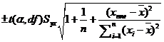 ; the additional term of 1 within the square root makes this
confidence interval wider than for the previous case.
; the additional term of 1 within the square root makes this
confidence interval wider than for the previous case.
The notes Regression Analysis – Confidence Level for a Measured X are more applicable when you are using a calibration curve to find x when y is measured.
