Spreadsheets - Functions

A function is a special prewritten formula that takes a value, or series of values, performs an operation, or series of operations, and returns a value, or values. Functions can simplify the creation/maintenance of a spreadsheet. Functions must follow a particular syntax, which are indicated below in monospaced font. Excel allows from 1-30 values (number1, number2, ...) in the parentheses after the function, although some functions (see PMT below) only require a specific number of values.

The Paste Function button  provides access to the Function Wizard, which will lead you through the steps required to create a formula. It also displays the value of the output as you are creating the formula, a useful feature when constructing complex formulas.

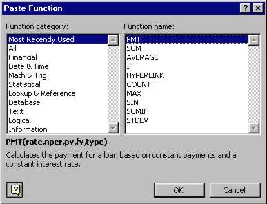
The first step in using the Function Wizard is to select the function you want to work with from the list presented. Broad categories appear on the left, and individual functions on the right.

After selecting the function, you will be presented with a dialog box allowing you to select/input the data values required. You can click the  button to select data values/ranges with the mouse, or enter the values directly into the appropriate fields. When you use choose to select your data, the selection box  appears below the formula bar and reflects your current selection.

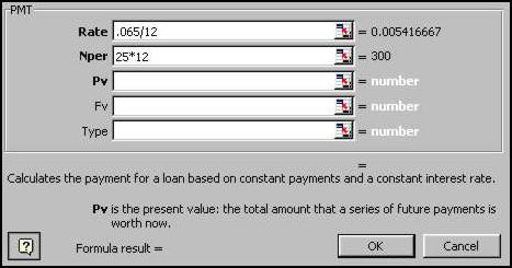
As you fill in required fields (the ones with bolded labels in the function wizard), their values appear in the appropriate fields in the wizard dialog box, and the complete formula is built in the formula bar . When you have filled in all the required fields, the result is shown at the bottom of the dialog box .

You are responsible for knowing how to apply the following commonly used functions.

SUM - Sum Function

Returns the SUM of all values in the list of arguments. The AutoSum button can be used to create a SUM function for a row or column of data. The function is inserted using the best guess for the associated row or column of data. If a range of columns or rows is selected, a SUM function will be created for each row or column in the selection.

AVERAGE - Average Function

Returns the average (arithmetic mean) of the arguments. Bear in mind that when calculating an average, Excel ignores empty cells, but does count cells containing the value 0.

MIN - Minimum Function

Returns the smallest number in the list of arguments. If a range of cells contains no numeric values, Excel will return a value of 0.

MAX - Maximum Function

Returns the maximum value in a list of arguments. If a range of cells contains no numeric values, Excel will return a value of 0.

Count - Count Function

Counts how many numbers are in the list of arguments (only numeric values are counted). Use COUNT to get the number of entries in a number field in a range or array of numbers. The COUNTA function is similar except it also counts cells with text values. For example,

If A3 contains "Sales," A4 contains "12/8/90," A6 contains "19," A7 contains "22.24

COUNT(A6:A7) equals 2

COUNT(A3:A7) equals 3

COUNTA(A3:A7) equals 4

SQRT - Square Root Function

Returns a positive square root of a number. If number is negative, SQRT returns the #NUM! error value.

ROUND - Round up Function

Rounds a number to a specified number of digits (num_digits).

• If num_digits is greater than 0, then number is rounded to the specified number of decimal places.
• If num_digits is 0, then number is rounded to the nearest integer.
• If num_digits is less than 0, then number is rounded to the left of the decimal point.

PMT - Payment Function

Returns the periodic payment (e.g. loan payment or mortgage) for an annuity (e.g. loan or mortgage) based on constant payments and a constant interest rate.

• Rate is the interest rate per period.
• Nper is the total number of payment periods in an annuity.
• Pv is the present value, the total amount that a series of future payments is worth now.
• Fv is the future value, or a cash balance you want to attain after the last payment is made. If fv is omitted, it is assumed to be 0 (the future value of a loan, for example, is 0).
• Type is the number 0 or 1 and indicates when payments are due. (0 or omitted, payment is at the end of the period, 1 it is at the beginning of the period

NOTE: The payments will be displayed in (parentheses), and in red, signifying a payment, or negative value.

For example, PMT(12%/12, 15*12, 100000) returns the monthly payments ($1,200.17) on a mortgage of $100,000, with an interest rate of 12%, and a period of 15 years. Multiplying this value by the period PMT(12%/12, 15*12, 100000)*(15*12) returns the total payed out at the end of the annuity.

The formula PMT(5%/12, 15*12, 0, 100000) returns the monthly payment ($374.13) required to save $100,000 over 20 years at an interest rate of 5%. Notice that the pv, or present value, place in the formula is filled in with a 0, as the current value of the savings is $0.

NOTE: To make the payment a positive value, simply make the present value negative.

For example, PMT(12%/12, 15*12, -100000) returns the monthly payments $1,200.17.

PV - Present Value Function

Returns the present value of an investment. The present value is the total amount that a series of future payments is worth now. For example, when you borrow money, the loan amount is the present value to the lender.

• Rate is the interest rate per period. For example, if you obtain an automobile loan at a 10% annual interest rate and make monthly payments, your interest rate per month is 10%/12, or 0.83%. You would enter 10%/12, or 0.83%, or 0.0083, into the formula as the rate.
• Nper is the total number of payment periods in an annuity. For example, if you get a four-year car loan and make monthly payments, your loan has 4*12 (or 48) periods. You would enter 48 into the formula for nper.
• Pmt is the payment made each period and cannot change over the life of the annuity. Typically, pmt includes principal and interest but no other fees or taxes. For example, the monthly payments on a $10,000, four-year car loan at 12% are $263.33. You would enter -263.33 into the formula as the pmt.
• Fv is the future value, or a cash balance you want to attain after the last payment is made. If fv is omitted, it is assumed to be 0 (the future value of a loan, for example, is 0). For example, if you want to save $50,000 to pay for a special project in 18 years, then $50,000 is the future value. You could then make a conservative guess at an interest rate and determine how much you must save each month.
• Type is the number 0 or 1 and indicates when payments are due.

Suppose you're thinking of buying an insurance annuity that pays $500 at the end of every month for the next 20 years. The cost of the annuity is $60,000 and the money paid out will earn 8%. You want to determine whether this would be a good investment. Using the PV function you find that the present value of the annuity is: PV(0.08/12, 12*20, 500, , 0) equals -$59,777.15 The result is negative because it represents money that you would pay, an outgoing cash flow. The present value of the annuity ($59,777.15) is less than what you are asked to pay ($60,000). Therefore, you determine this would not be a good investment.

FV - Future Value Function

Returns the future value of an investment based on periodic, constant payments and a constant interest rate.

• Rate is the interest rate per period.
• Nper is the total number of payment periods in an annuity.
• Pmt is the payment made each period; it cannot change over the life of the annuity. Typically, pmt contains principal and interest but no other fees or taxes.
• Pv is the present value, or the lump-sum amount that a series of future payments is worth right now. If pv is omitted, it is assumed to be 0.
• Type is the number 0 or 1 and indicates when payments are due. If type is omitted, it is assumed to be 0.

For example, you want to save money for a special project occurring a year from now. You deposit $1000 into a savings account that earns 6 percent annual interest compounded monthly (monthly interest of 6%/12, or 0.5%). You plan to deposit $100 at the beginning of every month for the next 12 months. How much money will be in the account at the end of 12 months? FV(0.5%, 12, -100, -1000, 1) equals $2301.40.

NPER - Number of Periods Function

Returns the number of periods for an investment based on periodic, constant payments and a constant interest rate.

• Rate is the interest rate per period.
• Pmt is the payment made each period; it cannot change over the life of the annuity. Typically, pmt contains principal and interest but no other fees or taxes.
• Pv is the present value, or the lump-sum amount that a series of future payments is worth right now.
• Fv is the future value, or a cash balance you want to attain after the last payment is made. If fv is omitted, it is assumed to be 0 (the future value of a loan, for example, is 0).
• Type is the number 0 or 1 and indicates when payments are due.

TODAY - Today Function

Returns the serial number of the current date. The serial number is the date-time code used by Microsoft Excel for date and time calculations. The default display format is the current default date format.

IF - If Function

Returns one value if logical_test evaluates to TRUE and another value if it evaluates to FALSE.

For example, IF(B2>C2,"Over Budget","OK") returns a value of Over Budget if the value in B2 is greater than that in C2, and OK if the value is lower.