Topic 10b - Priority Queues
You should already know what a queue is.
For those who don’t it is an ADT that store elements in the order they arrive.
Queues implement a FIFO (First In First Out) strategy.
However, elements need to be dealt in priority.
Activity
Do you have an idea of applications that requires to process some elements in priority without changing the global FIFO strategy?
In this topic we will discuss and implement a priority queue.
Model
A Priority Queue is an ADT that has the two following operations:
Insertion: Inserts a new element
DeleteMin: Find, return and remove the minimum element in the queue
As in many ADT you can add more operations.
Priority Queues have many applications, especially in greedy algorithms.
Simple implementations
We could think of a very simple implementation of a priority queue.
Activity
Discuss and come up with a simple implementation.
What is the complexity for insertion? Deletion?
When we say simple implementation, we usually think Linked List.
If we have a liked list:
Insertion: \(O(1)\)
DeleteMin: \(O(N)\)
Activity
Why is the deletion \(O(N)\)?
We want to delete the minimum element, thus to reduce the complexity we could use a sorted linked list.
If we consider a sorted list:
Insertion: \(O(N)\)
DeleteMin: \(O(1)\)
So, neither implementation is very efficient.
Note
The first implementation is better, as in average you’re inserting more than you’re deleting.
Binary Heap
Binary Heap is the most popular implementation of this ADT.
Usually we call priority queues heaps.
Structure
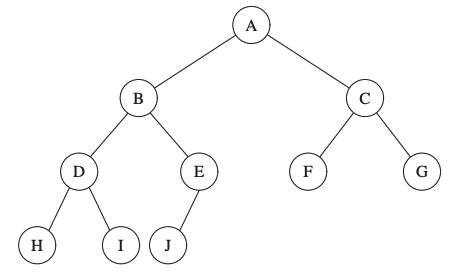
A heap is a binary tree that is completely filled with the possible exception of the bottom level.
Note
By definition it is a complete binary tree.
An example of a complete binary tree.
As a complete binary tree is regular, it is very easy to represent in an array.
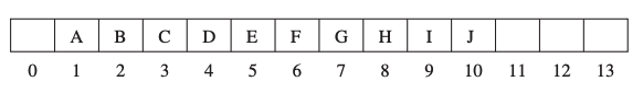
We can take any element in the array at position \(i\):
The left child is at position \(2i\).
The right child is at position \((2i + 1)\).
The parent is in position \(\lfloor i/2\rfloor\).
Header file
 1template<typename Comparable>
 2class BinaryHeap{
 3    public:
 4        BinaryHeap(int capacity = 100);
 5        BinaryHeap(const vector<Comparable>& items);
 6
 7        void insert(const Comparable& x);
 8        void deleteMin();
 9
10    private:
11        int curentSize;
12        vector<Comparable> array;
13};
Heap-Order Property
The Heap-Order property allows operations to be performed quickly.
To find the minimum element quickly, it needs to be at the root.
- The heap-order property:
For every node \(X\), the key in the parent of \(X\) is smaller than (or equal to) the key in \(X\), with the exception of the root.
The following is a good illustration of a heap:
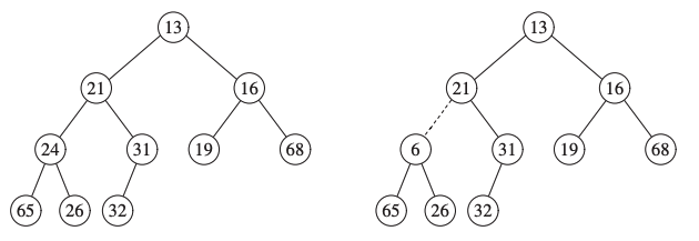
The left tree is a heap, the right tree is not.
Basic Operations
The two basic operations are simple to implement.
insert
To insert an element \(X\):
Create a hole in the next available location
If placing \(X\) in the hole violates the heap-order condition.
Put the parent’s hole in the hole, and \(X\) at the parent’s position.
Otherwise place \(X\) in the hole.
It continues until \(X\) can be placed in a hole.
Example
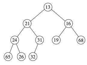
Consider the following tree.
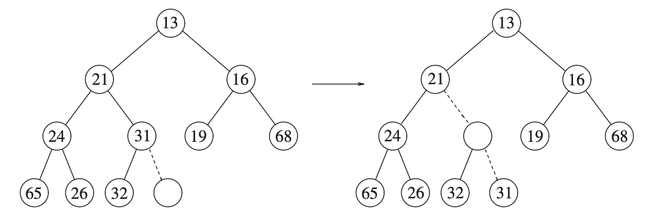
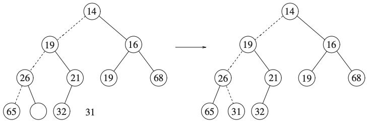
We want to insert the number \(14\).
We’re creating a hole for 14.
As it would break the heap-order property, we place the parent (\(31\)) in the hole instead.
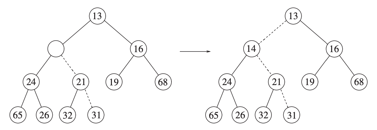
We continue the process.
Activity
Insert 5, 59 and 10 in the previous binary heap.
Draw the tree after each step.
Implementation
 1void insert(const Comparable& x){
 2    if (currentSize == array.size() - 1){
 3        array.resize(array.size() * 2);
 4    }
 5    int hole = currentSize++;
 6    Comparable copy = x;
 7
 8    array[0] = copy;
 9    for ( ; x < array[hole/2]; hole /= 2){
10        array[hole] = array[hole/2];
11    }
12
13    array[hole] = array[0];
14}
The time complexity of the insertion in the worst-case \(O(\log N)\).
deleteMin
Finding the minimum is easy, but removing it is hard.
When a minimum is removed, a hole is created.
We should place the last element in the heap \(X\) in the hole.
If we can place it, we’re done otherwise
We slide the smaller children in the hole.
We continue until \(X\) can be placed in the hole.
Example
Consider the previous tree.
We want to delete the number 13.
It creates a hole, 31 the last element cannot be inserted.
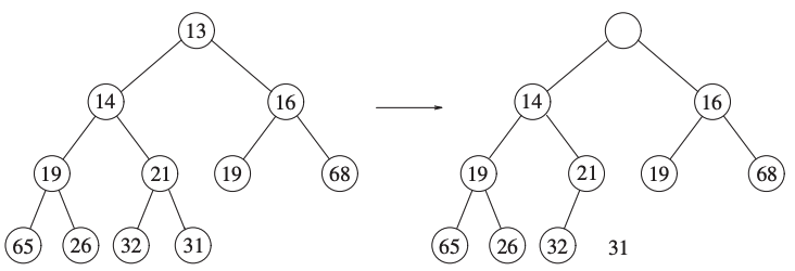
We’re move 14 up to fill the hole.
Inserting 31 would break the heap-order property, so we place the smaller children (19) in the hole instead.
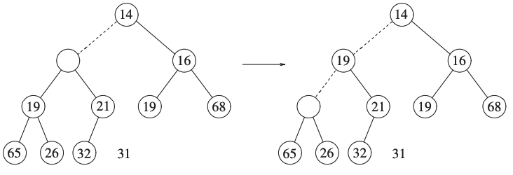
We continue the process.
We call this strategy percolating down.
Activity
Delete 14 and draw the tree after each step.
Implementation
 1Comparable deleteMin(){
 2    array[1] = array[currentSize--];
 3    percolateDown(1);
 4}
 5
 6void percolateDown(int hole){
 7    int child;
 8    Comparable tmp = array[hole];
 9
10    for ( ; hole*2 <= currentSize; hole = child){
11        child = hole * 2;
12        if ( child != currentSize && array[child + 1] < array[child]){
13            ++child;
14        }
15        if (array[child] < tmp){
16            array[hole] = array[child];
17        }
18        else{
19            break;
20        }
21
22    }
23    array[hole] = tmp;
24}
The time complexity in the worst-case is \(O(\log N)\).
In average it is also \(O(\log N)\).