Topic 13 - Graph Algorithms

Now we have the tools to see some graph algorithms.

Topological Sort

• A topological sort is an ordering of nodes in a directed acyclic graph.

• If there is a path from \(v_i\) to \(v_j\).

• Then \(v_j\) appears after \(v_i\) in the ordering.

Example

• Following an acyclic graph.

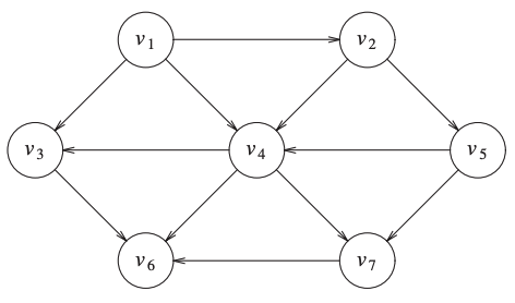
• An example of a topological ordering: \(v_1, v_2, v_5, v_4, v_7, v_3, v_6\).

Activity

• Give another topological ordering.

A Simple Algorithm

• We define the indegree of a vertex \(v\), as the number of edges \((u,v)\).

• A simple algorithm to find topological ordering is:

  • Find any vertex with an indegree of 0.

  • Remove it along with its edges.

  • Apply the strategy with another vertex.

• We obtain the following pseudocode:

void Graph::topsort()
{
    for (int counter = 0; counter < NUM_VERTICES; counter++){
        Vertex v = findNewVertexOfIndegreeZero();
        if (v == NOT_A_VERTEX){
            throw CycleFoundException();
        }
        v.topNum = counter;
        for each Vertex w adjacent to v{
            w.indegree--;
        }
    }
}

• Where findNewVertexOfIndegreeZero() scans the array of vertices looking for a vertex with indegree 0.

• If it returns NOT_A_VERTEX it indicates that the graph has a cycle.

• The complexity of this algorithm \(O(|V|^2)\).

A Second Algorithm

• The graph could be parsed, so checking each vertex could be a waste of time.

• A second way to make a topological sort is to place every vertex of indegree 0 in a queue.

• While the queue is not empty we remove one vertex.

• All the adjacent vertices have their indegree decremented.

Following a pseudo-code of the algorithm:

void Graph::topsort( )
{
    Queue<Vertex> q;
    int counter = 0;

    q.makeEmpty( );
    for each Vertex v
        if( v.indegree == 0 )
            q.enqueue( v );

    while( !q.isEmpty( ) )
    {
        Vertex v = q.dequeue( );
        v.topNum = ++counter; // Assign next number
        for each Vertex w adjacent to v
            if( --w.indegree == 0 )
                q.enqueue( w );
    }

    if( counter != NUM_VERTICES )
        throw CycleFoundException{ };
}

• The running time of this algorithm is \(O(|E|+|V|)\).

Activity

• Can you explain the running time?

• Apply this algorithm to the previous graph.

Shortest-Path Algorithms

• There are different shortest-path algorithms.

• But, they have common properties:

  • The input is a weighted graph.

  • The weight for each edge \((v_i, v_j)\) is a cost \(c_{i,j}\) to traverse the edge.

  • The cost of a path \(v_1v_2\dots v_N\) is \(\sum_{i=1}^{N-1}c_{i,i+1}\).

Activity

• What would be the cost of path in an unweighted graph?

• Consider the previous graph:

  • What is the cost of the path \(v_1, v_2, v_5, v_7\).

  • Do you have a shorter path from \(v_1\) to \(v_7\)?

Unweighted Shortest Paths

• Finding the shortest path in an unweighted graph is considering a weighted graph where all the edges have a cost of 1.

• It is minimizing the number of edges in the path.

A very simple algorithm is breadth-first search.

Breadth-First Search

The idea is to process vertices in layers.

Example

• Consider the previous unweighted directed graph.

• We want to apply breadth first to find the shortest path from \(v_1\) to \(v_6\).

• We obtain the following steps:

We start with the first node \(v_1\).

We check each arc leaving \(v_1\).

We continue until we find \(v_6\).

Activity

• Apply the algorithm to find the shortest path from \(v_4\) to \(v_1\).

First Implementations

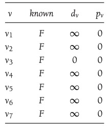
• First we create a table that will keep track of the algorithm progress.

• The table will keep track for each vertex:

  • its distance from \(s\) in \(d_v\).

  • the path \(p_v\).

  • if it was processed \(known\).

• An example of the table for the previous graph, with \(s=v_3\):

The pseudo-code is given below:

void Graph::unweighted( Vertex s )
{
    for each Vertex v
    {
        v.dist = INFINITY;
        v.known = false;
    }
    s.dist = 0;
    for( int currDist = 0; currDist < NUM_VERTICES; currDist++ )
        for each Vertex v
            if( !v.known && v.dist == currDist )
            {
                v.known = true;
                for each Vertex w adjacent to v
                if( w.dist == INFINITY )
                {
                    w.dist = currDist + 1;
                    w.path = v;
                }
            }
}

• The complexity of this algorithm is \(O(|V|^2)\).

Activity

• Is the algorithm efficient?

• If not, how would you improve it?

Dijkstra’s Algorithm

• Dijkstra’s algorithm is the general algorithm to solve the shortest path problem.

• It is a greedy algorithm. It solves a problem by selecting what seems the best solution at each step.

• The information that we keep:

  • Each vertex is either known or unknown.

  • A distance \(d_v\) is kept for each vertex.

The idea

• It proceeds in stages.

• At each stage, Dijkstra selects a vertex \(v\) which has the smallest \(d_v\) among all unknown vertices.

• It becomes the new shortest path from \(s\) to \(v\).

• Then it updates the values of \(d_w\).

  • In the unweighted case \(d_w = d_v + 1\).

  • In the weighted case \(d_w = d_v + c_{v,w}\).

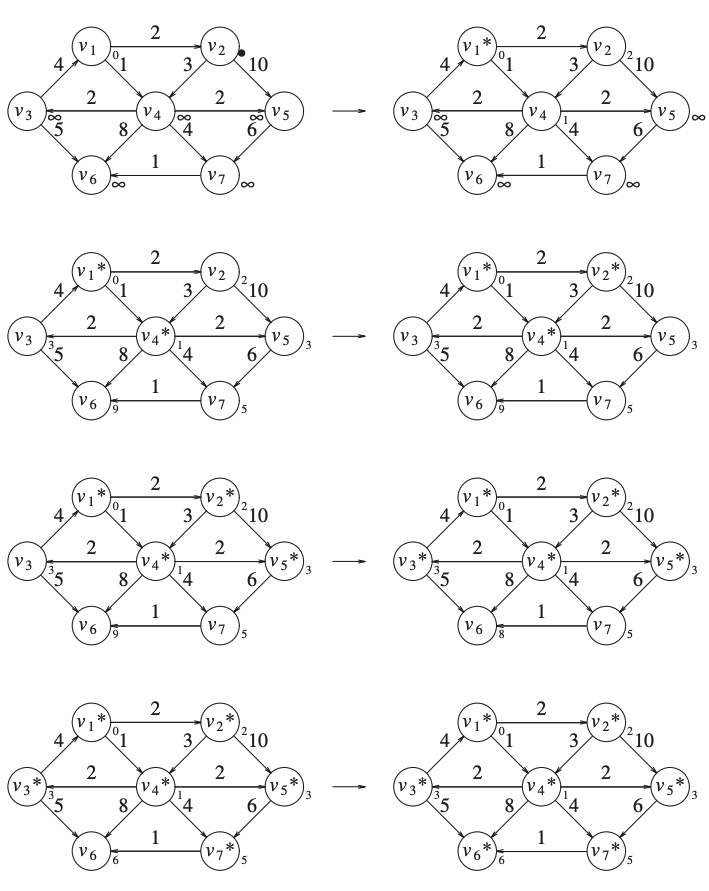
Example

• We will illustrate the algorithm with an example.

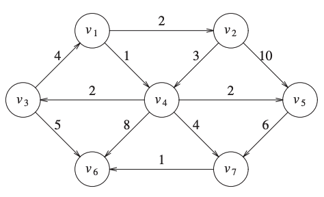
• Consider the following graph:

• Now we have the initial configuration:

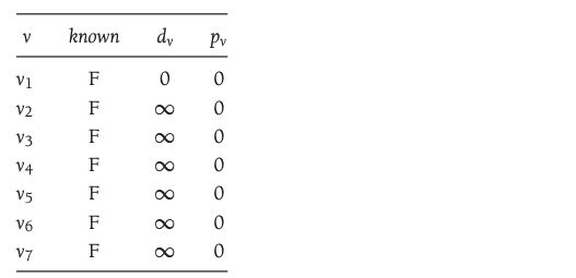
• If we assume that \(s = v_1\) is our initial node.

• Then we select \(v_1\), we put it to known.

• \(v_2\) and \(v_4\) are adjacent, so we put their distances from \(v_1\).

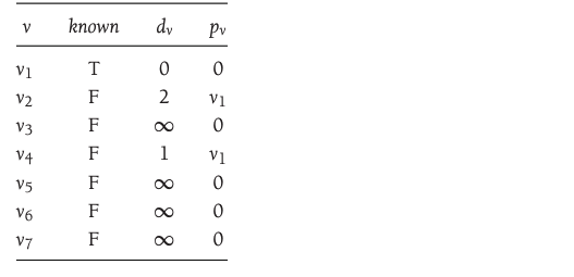
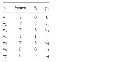
• \(v_4\) has the smallest distance, so it is the next selected node.

• It is marked as known.

• \(v_3, v_5, v_6\) and \(v_7\) are adjacent.

• We update them accordingly.

• Next \(v_2\) is selected.

• \(v_4\) is adjacent but already known, so no work is done on it.

• \(v_5\) is adjacent but not adjusted, because going through \(v_2\) is \(12\) and a path of length 3 is already known.

• The next vertex selected is \(v_5\).

• \(v_7\) is the only one adjacent, but it is not adjusted.

• Then, \(v_3\) is selected and \(v_6\) is adjusted to 8.

• We then select \(v_7\).

• We update \(v_6\) to 6.

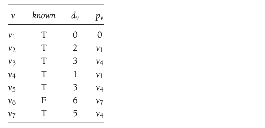
• Finally we select \(v_6\) and stop there.

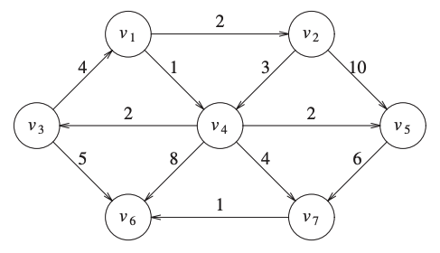
• We can also show that graphically.

Implementation

• The implementation is done in two parts.

• The first part is the definition of the node:

/**
* PSEUDOCODE sketch of the Vertex structure.
* In real C++, path would be of type Vertex *,
* and many of the code fragments that we describe
* require either a dereferencing * or use the
* -> operator instead of the . operator.
*/
struct Vertex
{
    List adj; // Adjacency list
    bool known;
    DistType dist; // DistType is probably int
    Vertex path; // Probably Vertex *, as mentioned above
    // Other data and member functions as needed
};

• And the algorithm directly:

void Graph::dijkstra( Vertex s )
{
    for each Vertex v
    {
        v.dist = INFINITY;
        v.known = false;
    }
    s.dist = 0;
    while( there is an unknown distance vertex )
    {
        Vertex v = smallest unknown distance vertex;
        v.known = true;
        for each Vertex w adjacent to v
        {
            if( !w.known )
            {
                DistType cvw = cost of edge from v to w;
                if( v.dist + cvw < w.dist )
                {
                    // Update w
                    decrease( w.dist to v.dist + cvw );
                    w.path = v;
                }
            }
        }
    }
}

• This algorithm is running in \(O(|E|+|V|^2) = O(|V|^2)\).

• If the graph is too dense, the algroithm is slow.

• With few modifications we can make it run in \(O(|E|\log |V|)\).

Network Flow Problems

• Suppose a directed graph \(G=(V,E)\).

• Each edge has a capacity of \(c_{v,w}\).

• We could consider that the capacity is the amount of water that could flow through a pipe.

Definition

• In a network flow problem, the graph contains two nodes:

  • \(s\) called the source.

  • \(t\) called the sink.

• \(c_{v,w}\) is the maximum unit of “flow” that can pass.

• At any vertex \(v\) (not being \(s\) or \(t\)) the total incoming flow must be equal to the total flow exiting the node.

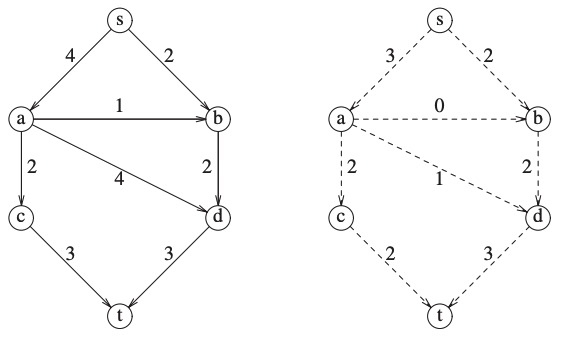
• The maximum flow problem is to determine the maximum flow amount that can pass from \(s\) to \(t\).

• The following graph has a maximum flow of 5:

Activity

• Do you have any real application of this problem?

• Can you increase the flow in this graph?

• Can you prove it?

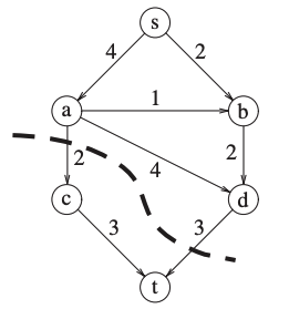
• If we cut the graph in two parts:

  • A part containing \(s\) and few nodes.

  • A part containing \(t\) and few nodes.

• The capacity leaving the first part is the maximum flow:

A simple Maximum-Flow algorithm

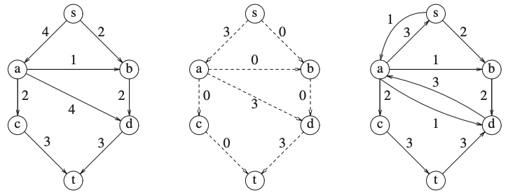
• We start with our graph \(G\) and construct a flow graph \(G_f\).

• \(G_f\) is the flow that has been attained at any stage.

• Initially all edges in \(G_f\) has no flow.

• At the end \(G_f\) should contain the maximum flow.

• We also construct \(G_r\), the residual graph.

• \(G_r\) contains for each edge how much flow can be added.

How does it work?

• At each stage, we find a path in \(G_r\) from \(s\) to \(t\).

• The minimum edge on the path is the amount of flow that is added to every edge on the path in \(G_f\).

• We recalculate \(G_r\) and we add an opposite edge with the same capacity.

• When we find no path from \(s\) to \(t\) in \(G_r\) we stop.

Example

• If we apply it to the previous graph.

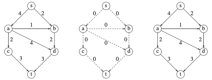
• Now we find a path:

• And we continue:

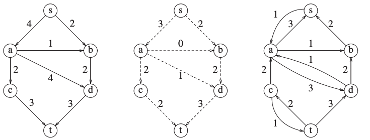
• You can see that we changed a previous flow.