9. Hash Table without Linked Lists
In the previous topic, we saw how to create a hash table using the separate chaining, meaning using linked lists to store elements that have the same hash.
The only issue is the running time of adding and searching in the linked list.
9.1. Idea
The linked lists are used in case of collision.
To remove the linked list, we need to deal with the collision differently.
Consider the following:
You have an element \(x\).
You hash the element \(h = hash(x)\)
You check if the cell \(h\) is occupied or not.
If it is, you have a collision, then you check \(h + 1\).
You continue until one cell is empty.
It is called Probing Hash Tables.
More formally, we check a cell \(h_i(x)\) defined as:
where \(f\) is the collision resolution function and \(f(0) = 0\).
Of course, we can use different collision resolution function.
Important
The size of the table must be larger than with separate chaining tables.
9.2. Linear Probing
In linear probing, \(f\) is a linear function:
It’s very simple to understand, so we will take an example to illustrate it.
Example
Consider the hash function \(hash(x) = x\).
Consider a table of size 10.
Now we want to insert the following element \(\{89, 18, 49, 58, 69\}\).
For each element we calculate \(h_i(x) = (x + f(i))\mod 10)\).
We obtain the following result:
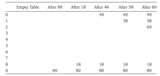
As long as the table is large enough we can always find an empty cell.
However, the running time can be quite large.
Activity
Why can the running time grow very quickly with linear probing?
This problem is accentuated with the primary clustering effect.
It occurs when block of occupied cells start forming.
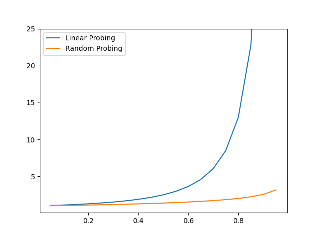
It is possible to calculate the average number of probes required using a linear probing strategy and a random probing strategy.
Linear probing (insertion): \(\frac{1}{2}(1+ \frac{1}{(1-\gamma)^2})\).
Random probing (insertion): \(\frac{1}{\gamma}\ln \frac{1}{1-\gamma}\)
We can see that the number of prob before finding a cell to insert a new element grows quickly with the load factors:
9.3. Quadratic Probing
Linear probing is not optimal due to the primary clustering.
Quadratic probing eliminates this issue.
Obviously, the collision function is quadratic, usually \(f(i) = i^2\) is used.
Activity
Take the previous example and the new collision function and show what is the state of the table after each insertion.
Are we avoiding the primary clustering issue?
With quadratic probing there is no guarantee of finding an empty cell once the table gets more than half full!
This is because the at most half of the table can be used as alternative locations.
It leads us to the following.
Theorem
If quadratic probing is used, and the table size is prime, then a new element can always be inserted if the table is at least half empty.
Proof
Let \(TableSize\) be an odd prime greater than 3.
We show that:
\(\lceil TableSize/2\rceil\) alternative locations are all distinct.
Two of these locations are \(h(x)+i^2 \mod TableSize\) and \(h(x)+j^2 \mod TableSize\), where \(0\leq i, j\leq \lfloor TableSize/2 \rfloor\).
(Proof by contradiction):
Suppose that the locations are the same but \(i\neq j\), then:
Since \(TableSize\) is prime, either \((i-j)\) or \((i+j)\) is equal 0.
Since \(i\) and \(j\) are distinct, the first option is impossible.
Since \(0\leq i, j\leq \lfloor TableSize/2 \rfloor\), the second option is impossible.
If at most \(\lfloor TableSize / 2 \rfloor\) positions are taken, then an empty spot can always be found.
9.3.1. Implementation
The implementation is in the most part straightforward with the exception of the deletion.
If we remove an element that caused a collision, finding the elements that collided will fail.
We will consider each cell to have three states:
Active
Empty
Deleted
private final Entry<K, V> DELETED = new Entry<>(null, null);
So we define the interface of the class as:
HashTable with probing
 1/** Hash table implementation using open addressing. */
 2public abstract class HashTableOpen<K, V> extends HashTable<K, V> implements KWHashMap<K, V> {
 3
 4
 5    // Data Fields
 6    protected Entry<K, V>[] table;
 7    private static final int START_CAPACITY = 101;
 8    private double LOAD_THRESHOLD = 0.75;
 9    private int numKeys;
10    private int numDeletes;
11    private final Entry<K, V> DELETED = new Entry<>(null, null);
12
13    // Constructor
14    public HashTableOpen() {
15        table = new Entry[START_CAPACITY];
16    }
17    /**
18     * Return the value associated to the key.
19     *
20     * @param key the key
21     * @return the value or null if the key is not present.
22     */
23    @Override
24    public V get(K key) {
25    }
26
27    /**
28     * Returns true if this table contains no key-value mappings.
29     *
30     * @return true or false
31     */
32    @Override
33    public boolean isEmpty() {
34    }
35
36    /**
37     * Associated the value with the speficied key.
38     *
39     * @param key   the key
40     * @param value the value
41     * @return Returns the previous value associated with the specified key, or null if there was no mapping for the key
42     */
43    @Override
44    public V put(K key, V value) {
45    }
46
47    /**
48     * Remove the mapping for this key from the table if it is present.
49     *
50     * @param key the key
51     * @return Returns the previous value associated with the specified key, or null if there was no mapping.
52     */
53    @Override
54    public V remove(K key) {
55    }
56
57    /**
58     * Return the size of the table
59     *
60     * @return the size
61     */
62    @Override
63    public int size() {
64        return numKeys;
65    }
66
67    /** Finds either the target key or the first empty slot in the
68     search chain using linear probing.
69     pre: The table is not full.
70     @param key The key of the target object
71     @return The position of the target or the first empty slot if
72     the target is not in the table.
73     */
74    protected int find(K key) {
75    }
76
77    /** Expands table size when loadFactor exceeds LOAD_THRESHOLD
78     post: The size of the table is doubled and is an odd integer.
79     Each nondeleted entry from the original table is reinserted into the expanded table.
80     The value of numKeys is reset to the number of items actually inserted; numDeletes is reset to 0.
81     */
82    private void rehash() {
83    }
84
85
86}
9.3.1.1. get
The function contains require one other functions:
find: find the cell of the element (deal with the collision, etc.)
The functions get is very easy to implement:
 1    /**
 2     * Return the value associated to the key.
 3     *
 4     * @param key the key
 5     * @return the value or null if the key is not present.
 6     */
 7    @Override
 8    public V get(K key) {
 9        // Find the first table element that is empty
10        // or the table element that contains the key.
11        int index = find(key);
12        // If the search is successful, return the value.
13        if (table[index] != null)
14            return table[index].getValue();
15        else
16            return null; // key not found.
17    }
For find we need to proceed by steps:
Initialize the offset aka \(f(1)\).
Calculate the current position by calculating the hash of the element
While the position is not empty and it is not the element we’re looking for:
we had the offset to the hash.
we increment the offset, using the quadratic collision function \(f(i) = f(i-1) + 2*i -1\).
If the current position is greater than the size subtract the size.
Activity
Implement the function
find.
1public class HashTableOpenQuad<K, V> extends HashTableOpen<K, V> implements KWHashMap<K, V>{
2
3    @Override
4    protected int find(K key) {
5    }
6
7}
9.3.1.2. put
To insert we do the following:
Find the position of the new element.
Put the element at the position
If the number of element (inserted and deleted) is greater than the size of the table, rehash.
Activity
Implement the function
put.
9.3.1.3. remove
Very similiar to insert:
Find the position of the element to delete.
Put the element state to
DELETE.return the old value.
9.4. Double Hashing
The last collision resolution function is double hashing.
The idea is simple, we apply a second hashing function inside the hashing function.
A popular function is :
Note, that we apply the second hash function inside the probe function.
The second hash function needs to be selected carefully.
We need to ensure that all cells can be probed.
It requires that \(TableSize\) is prime.
After that a simple function as:
works well, if \(R\) is a prime number smaller than \(TableSize\).
Important
If double hashing is implemented correctly, then the expected number of probes is almost the same as for a random collision function.
9.5. Rehashing
If the table gets too full, the running time for the operations will increase.
A solution is
to build another table that is around twice the size (prime number)
scan the original hash table
compute the new hash value for each (nondeleted) element and insert it in the new table.
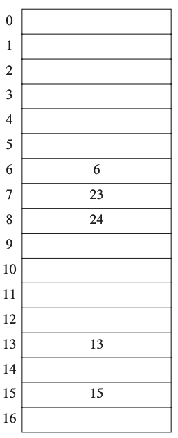
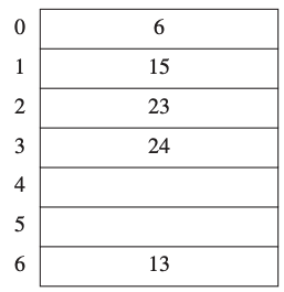
Example
Consider the following table.
The hash function is \(h(x) = x \mod 7\).
It is more than half full.
So we need to rehash the table.
We created a new table around twice the size (closest prime number).
Every value of the previous table have been inserted using the new hash function \(h(x) = x \mod 17\).