8. Temporal-Difference Learning

• We covered the fundamentals to understand reinforcement learning.

• One central methods for reinforcement learning is called Temporal-Difference (TD) learning.

• TD learning is composed of:

  • Dynamic programming

  • Monte Carlo methods.

8.1. TD Prediction

Activity

• Following is the update done by Monte Carlo methods?

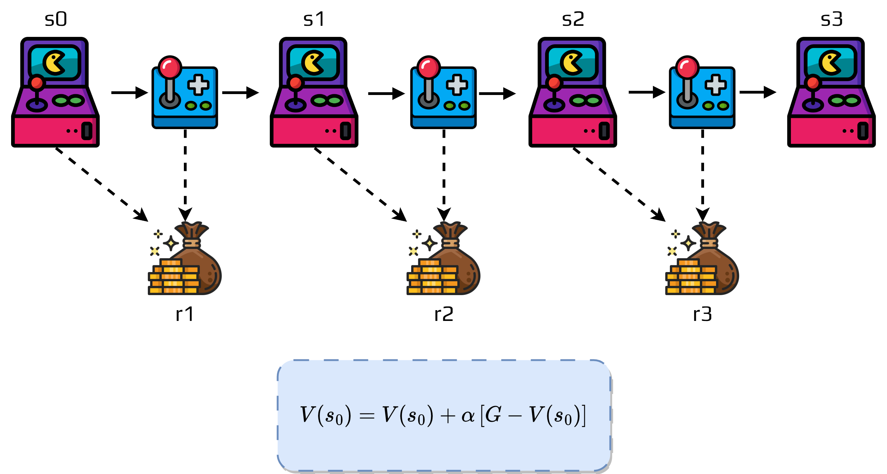
• What is the disadvantage?

• TD works differently.

  • TD forms a target at time \(t+1\).

  • We use the reward \(r_{t+1}\) and the current estimate \(V(s_{t+1})\) to update \(V(s_{t})\).

• The update is done as:

\[V(s_t) \leftarrow V(s_t) + \alpha\left[ r_{t+1} + \gamma V(s_{t+1}) - V(s_t) \right]\]

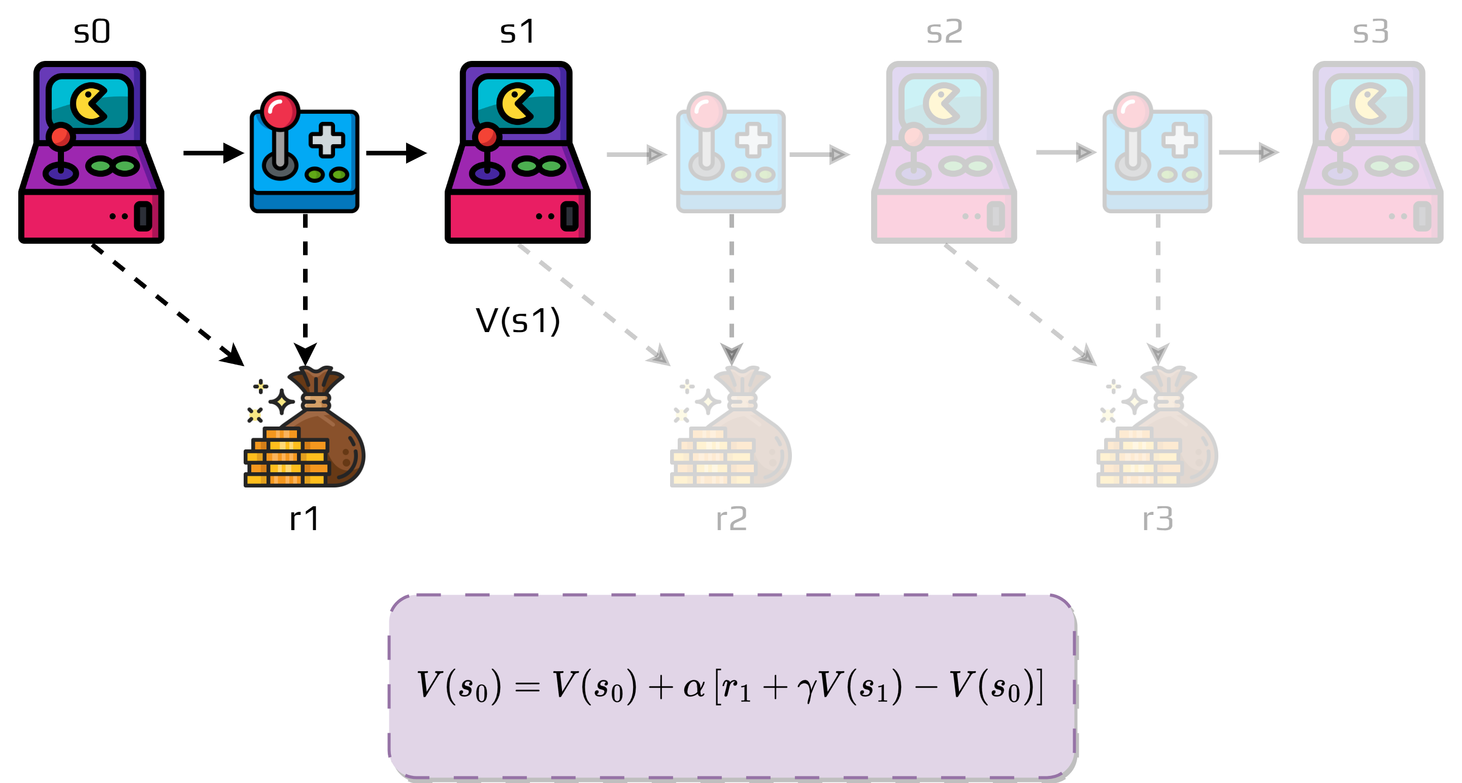
• This TD method is called TD(0).

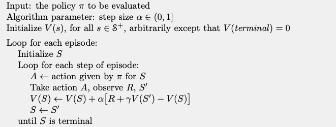
• We can write a very simple algorithm to evaluate the policy:

Algorithm TD(0)

Activity

• What major differences can you see between this algorithm and Monte Carlo?

• The TD target is an estimate for two reasons:

  1. The expected value \(V(s')\) is sampled.

  2. It uses the current estimate \(V(s)\).

• Moreover \(\left[ r + \gamma V(s') - V(s) \right]\) can be seen as an error.

  • It measures the difference between the estimated value \(V(s_t)\) and the better estimate \(r + \gamma V(s')\).

Important

It is called the TD error:

\[\delta_t = r_{t+1}+\gamma V(s_{t+1}) - V(s_t)\]

The TD error depends on the next state and next reward, so it’s not available until \(t+1\).

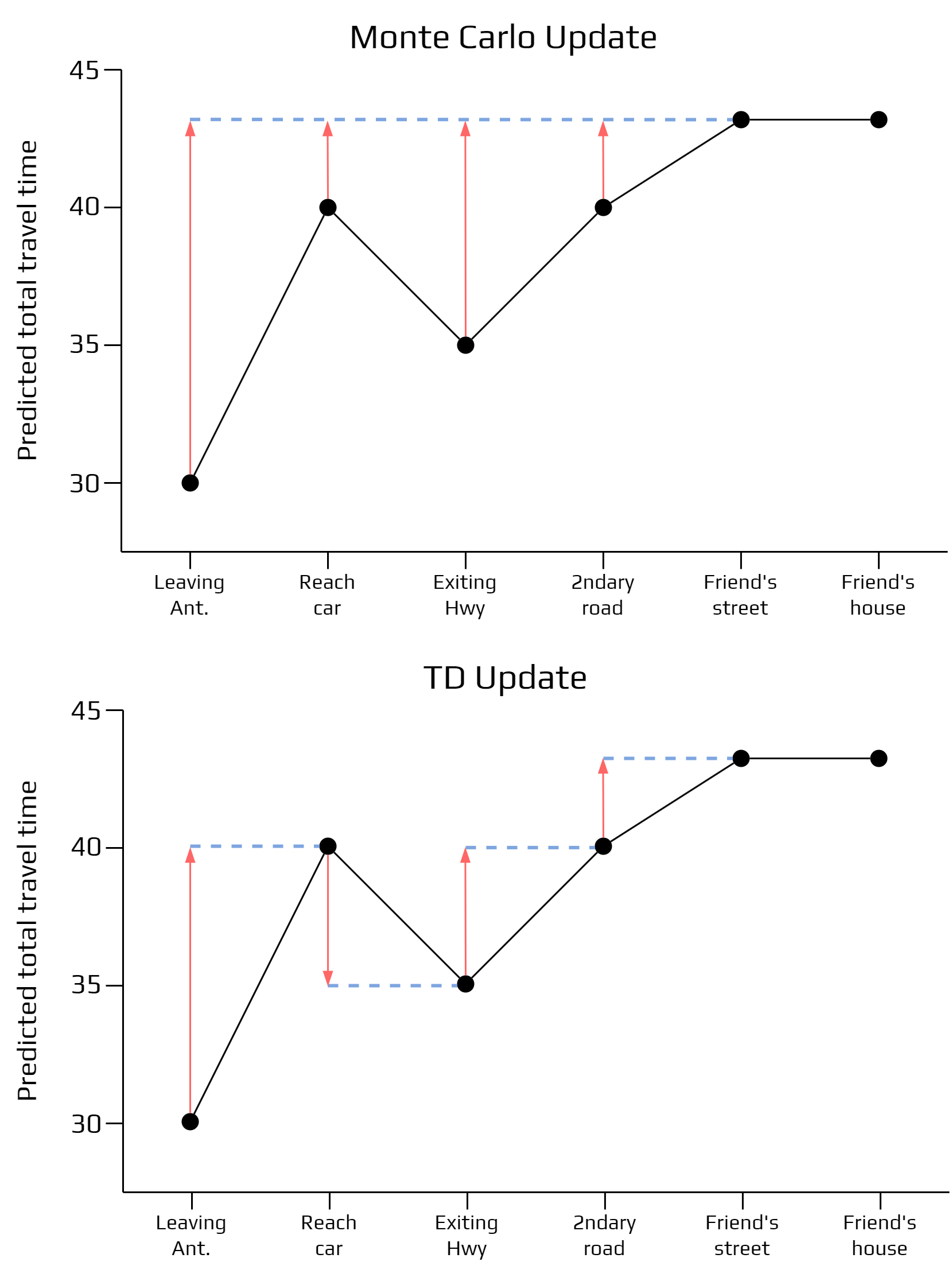
Example

• Some days as you drive to your friend’s house, you try to predict how long it will take to get there.

• When you leave town, you note the time, the day of week, the weather, and anything else that might be relevant.

• The following table summarizes what happened:

• If you apply, Monte Carlo and TD learning you would obtain this:

What are the advantage of TD learning?

• TD methods do not require a model of the environment, of the reward and transition function.

• An advantage over Monte Carlo methods is that they are online and fully incremental.

8.2. SARSA: On-Policy TD learning

• Now that we can estimate a policy, we can calculate the policy.

• TD methods we also need to trade off exploration or prediction.

• For on-policy methods we must estimate \(q_\pi(s,a)\) for all states \(s\) and actions \(a\).

Activity

• Why do we need to use the pair state-action?

• Concretely the update function becomes:

\[q(s,a) = q(s,a) + \alpha\left[ r_{t+1} + \gamma q(s_{t+1}, a_{t+1}) - q(s_t, a_t) \right]\]

• This update utilize every element of the transition \((s_,a_t,r_{t+1},s_{t+1},a_{t+1})\).

• This algorithm is called Sarsa and can be written as:

SARSA

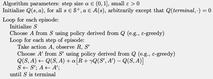
Note

• The action selection is important to have a good ratio between exploration and prediction.

• The strategies seen in previous topics can be used freely.

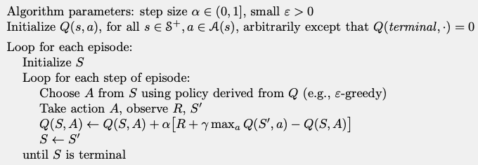
8.3. Q-Learning: Off-policy TD learning

• The off-policy learning algorithm called Q-Learning is old (1989).

• The update function is:

\[q(s_t, a_t) = q(s_t, a_t) + \alpha\left[ r_{t+1} + \gamma\max_{a'} q(s_{t+1}, a')- q(s_t, a_t) \right]\]

• In this case it approximates \(q^*\).

Q-Learning Algorithm

Activity

• Discuss the difference between these two algorithms.