7. Monte Carlo Methods
Dynamic programming is a method to calculate the optimal policies.
One issue with dynamic programming is that it requires complete knowledge about the environment.
In some problems we don’t assume complete knowledge.
To calculate a policy without this knowledge, the agent can only use its experience.
The experience comes from the interaction of the agent with the environment.

Important
A model is still required, but a full transition function is not.
7.1. Monte Carlo Prediction
The idea is simple:
We need to estimate \(v_\pi(s)\).
We consider all the trajectories from the initial state to the end state, called episodes.
Each occurrence of \(s\) in an episode is called a visit.
\(v_\pi(s)\) is the average of the returns of all the visits to \(s\).
Now we can put that in an algorithm.
Algorithm
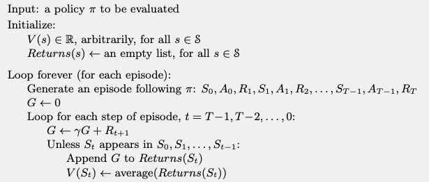
This algorithm converges to \(v_\pi(s)\) as the number of visits to \(s\) goes to infinity.
Activity
Consider the following episode.

We can see that one state is visited twice.
How do you calculate the return \(G\) for this state?
7.2. Mont Carlo Estimation of Action Values
Activity
How can you apply Monte Carlo methods when you don’t have a model?
How do we estimate the policy?
In this case we apply this method to a state-action pair.
Concretely, we want to estimate \(q^*(s,a)\).
We average the returns for each pair state-action.
Activity
Discuss what problems occur with this method.
All the actions need to be visited.
It is similar to the multi-armed bandit problem.
Balancing exploration/exploitation.
Note
The methods seen in the multi-armed bandit can be used.
7.3. Monte Carlo Control
We have all the tools to use Monte Carlo methods.
We can estimate the value function, now we need to improve the policy.
We consider two types of methods:
The on-policy control methods.
The off-policy control methods.
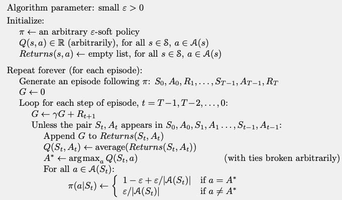
7.3.1. On-policy Method
In this method, the agent has a soft policy:
It starts with \(\pi(a|s) >0\), \(\forall s\in S, \forall a\in A\).
Gradually shift to a deterministic optimal policy.
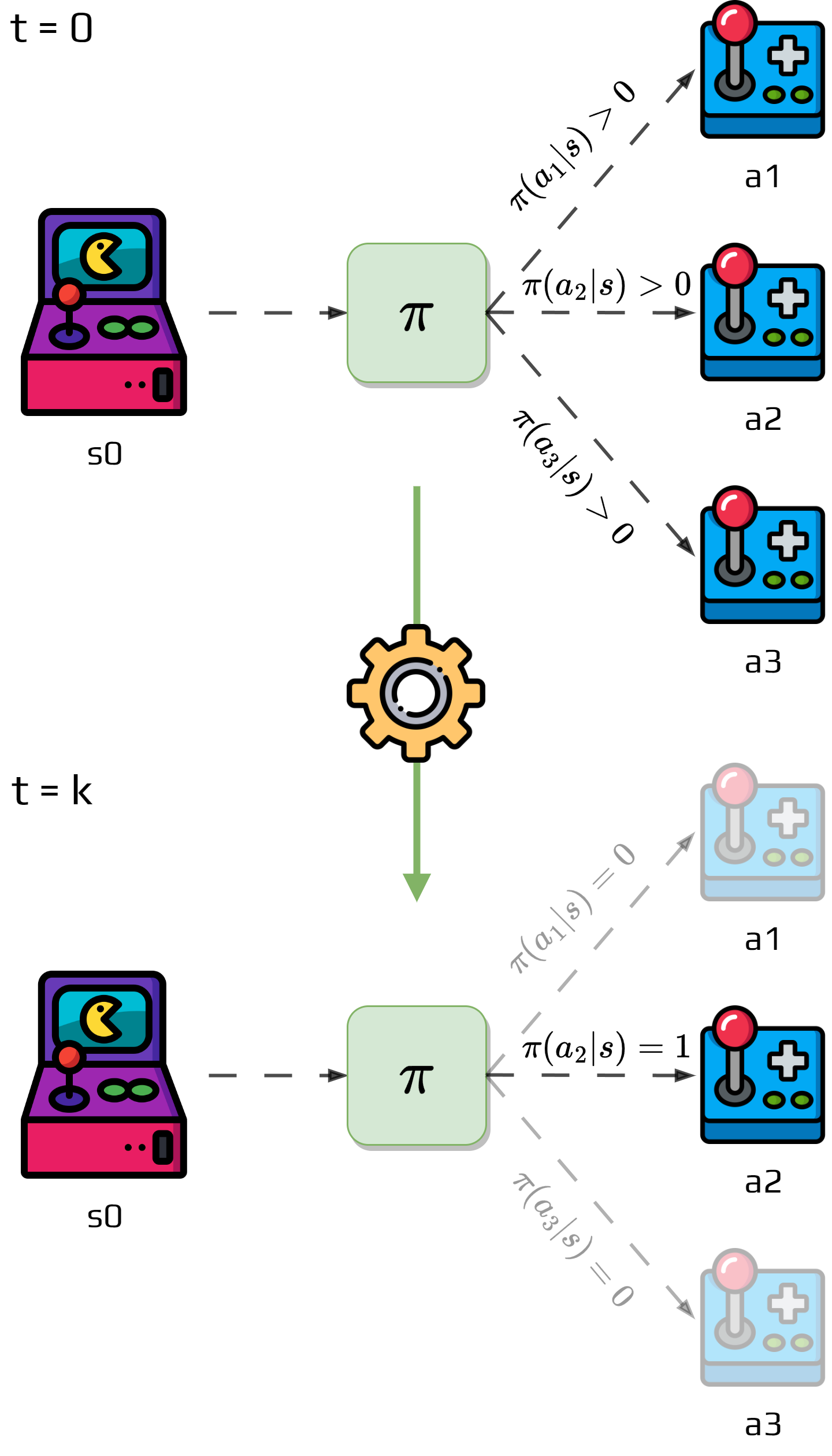
The one we will see is the \(\epsilon\)-greedy policy.
Nongreedy actions are given minimal probability of selection \(\frac{\epsilon}{|A|}\).
The greedy action gets the remaining probability \(1 - \epsilon+\frac{\epsilon}{|A|}\).
Algorithm
Activity
Make sure you understand the algorithm.
This algorithm guarantee that for any \(\epsilon\)-soft policy \(\pi\), any \(\epsilon\)-greedy with respect to \(q_\pi\) is guaranteed to be better than or equal to \(\pi\).
Proof
It is assured by the policy improvement theorem.:
Thus, by the policy improvement theorem \(\pi'\geq\pi\).
It achieves the best policy among the \(\epsilon\)-soft policies.
7.3.2. Off-policy Monte Carlo methods
On-policy methods learn action values for a near-optimal policy.
The exploratory part of the methods always generate a small number of less optimal actions.
Another approach is to use two policies:
One that is learned and that becomes the optimal policy.
The other that contains the exploratory component.
The learned policy is called the target policy.
The other policy is called the behavior policy.
We can summaries the two methods as:
On-Policy |
Off-Policy |
Generally, simpler |
|
7.3.2.1. Prediction problem
Consider the following problem:
Both policies are fixed and we just try to estimate \(v_\pi\).
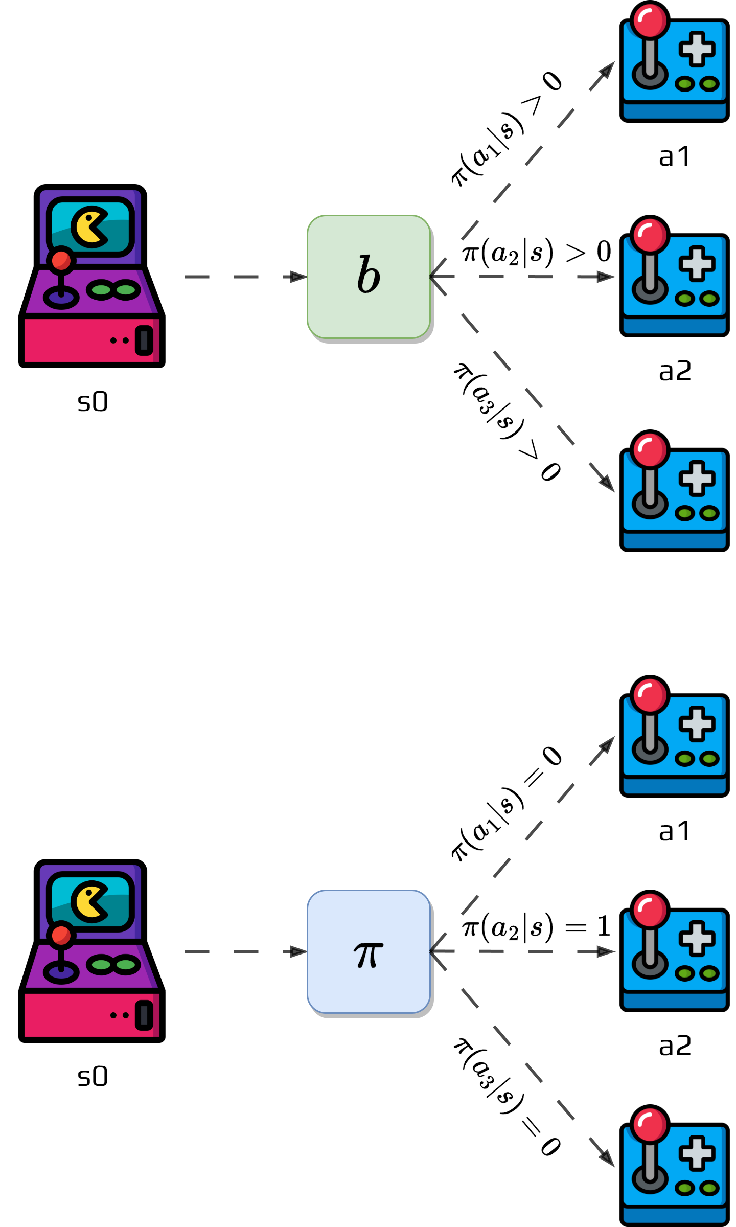
We don’t have \(\pi\); only episodes generated by another policy \(b\) with \(\pi\neq b\).
\(\pi\) is the target policy and \(b\) is the behavior policy.
We want to use the episode generated by \(b\) to estimate \(\pi\).
To do it, we require:
Every action taken under \(\pi\) is also taken under \(b\).
Meaning, \(\pi(a|s)>0\) implies \(b(a|s)>0\).
It is called the assumption of coverage.
Activity
Why is this assumption important?
Now we need to see how we estimate the action values.
Off-policy methods utilize importance sampling.
It takes the returns of the trajectories.
Weights them relatively to their probability of occurring in both policies.
It is called importance-sampling ratio.
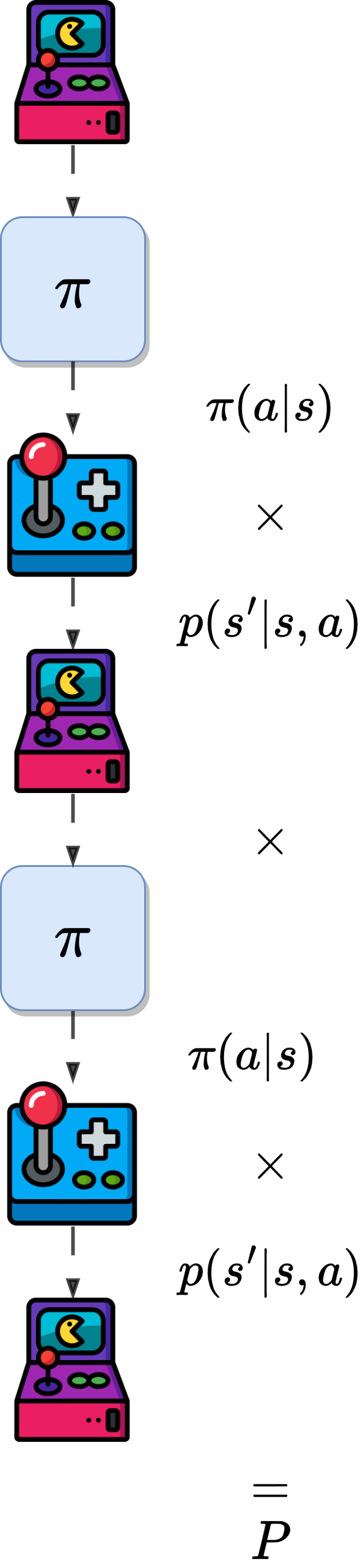
Giving a starting state \(s_t\).
The probability of the subsequent state-action trajectory \(a_t,s_{t+1},a_{t+1},\dots,s_T\) occurring under \(\pi\) is:
\[\begin{split}\begin{aligned} &P(a_t,s_{t+1},a_{t+1},\dots,s_T|s_t,a_{t:T-1}\sim \pi)\\ &= \prod_{k=t}^{T-1}\pi(a_k|s_k)p(s_{k+1}|s_k,a_k) \end{aligned}\end{split}\]
The importance-sampling ratio is:
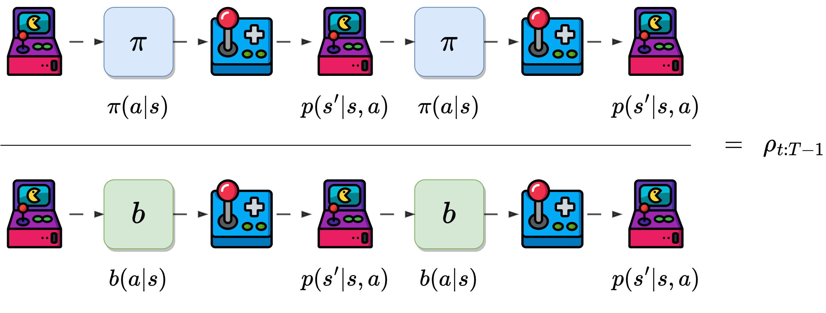
Important
The importance sampling ratio ends up depending only on the two policies and the sequence not on the MDP.
We wish to estimate the expected returns under the target policy \(\pi\).
We have the returns \(G_t\) under \(b\).
The expectation \(\mathbb{E}[G_t|s_t=s]=v_b(s)\) cannot be averaged to obtain \(v_\pi\).
We use the ratio \(\rho_{t:T-1}\) to transform the returns to have the right expected value:
Concretely:
We define \(\mathcal{T}(s)\), the set of all times steps in which state \(s\) is visited.
We use it to obtain the value function update:
Note
It considers that we have the entire trajectories to update it.
However, we can modify it to have an incremental implementation.
Update after each episode.
Suppose we have a sequence of returns \(G_1, G_2, \dots, G_{n-1}\)
All starting in the same state,
And with corresponding random weight \(W_i = \rho_{t_i:T(t_i)-1}\)
We want to calculate:
We also need to maintain for each state the cumulative sum \(C_n\) of the weights given the first \(n\) returns.
The update rule for \(V_n\) is:
and
Important
We saw this in the multi-armed bandit!
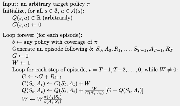
We can now write an algorithm:
Off policy prediction algorithm
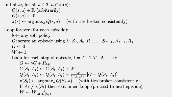
7.3.2.2. Off-policy control
We can estimate the value of a policy using an off-policy Monte Carlo method.
To caulculate the optimal policy using an off-policy method:
We consider the policy \(\pi\) we want to calculate to be a greedy policy.
After each update of the value function, we assign the best action to the policy.
The algorithm can be written as:
Algorithm