10. Eligibility Traces
Until now, we saw two main methods to do reinforcement learning:
Monte-Carlo methods
Temporal-difference methods
Activity
What is the main difference between these two methods?
Eligibility trace is a mechanism of reinforcement learning that unifies both methods.
A popular algorithm is TD(\(\lambda\)), where \(\lambda\) refers to the eligibility traces.
This mechanism is a short-term memory vector called eligibility trace \(\mathbf{z}_t\in \mathbb{R}^d\).
It is a parallel to the long-term weight vector \(\mathbf{w}_t\).
The idea:
When a component of \(\mathbf{w}_t\) is used to estimate a value,
The corresponding components of \(z_t\) is increased,
Then start to fade away.
The trace-decay \(\lambda\in [0,1]\).
There are advantages compared to other methods:
A single trace error is required to do the update.
The learning is done at each step.
The learning can affect the behavior of the following step.
10.1. The \(\lambda\)-return
Consider the return on \(n\)-steps:
\[G_{t:t+n} = r_{t+1} + \gamma r_{t+2} + \dots + \gamma^{n-1}r_{t+n} + \gamma^n\hat{v}(s_{t+n}, \mathbf{w}_{t+n-1}), 0\leq t \leq T-n\]where \(\hat{v}(s,\mathbf{w})\) is the approximate value of state \(s\) given weight vector \(\mathbf{w}\).
Another valid update can be done toward any average of \(n\)-steps returns.
Example
Consider a 4-steps return.
The update can be done toward a target that is half of a two-step return and half of a four-step return:
The update can be represented graphically like this:
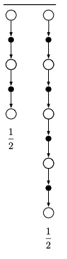
There are lots of ways to do a compound update, but it can only be done when the longest components update is complete.
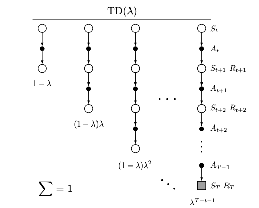
TD(\(\lambda\)) algorithm is a particular way of averaging \(n\)-steps updates.
Each step is weighted proportionally to \(\lambda^{n-1}\) (where \(\lambda\in [0,1]\))
Then it is normalized by a factor of \(1-\lambda\).
The resulting updated is called \(\lambda\)-return and is defined by:
The weight fades by \(\lambda\) with each additional step.
After a terminal state all subsequent \(n\)-steps returns are equal to the conventional return \(G_t\).
The following diagram represents this update:
Activity
Why are we normalizing the average?
Try to show that after the \(n\).
10.2. TD(\(\lambda\))
TD(\(\lambda\)) is one of the oldest and used algorithms in reinforcement learning to evaluate a policy.
Remember we said that it uses an eligibility trace \(\mathbf{z}_t\).
It has the same number of components that \(\mathbf{w}\).
In TD(\(\lambda\)):
The eligibility trace vector is initialized to zero at the beginning of the episode.
Then incremented on each time step by the value gradient and fades away by \(\gamma\lambda\):
\[\begin{split}\begin{aligned} \mathbf{z}_1 &= \mathbf{0}\\ \mathbf{z}_t &= \gamma\lambda\mathbf{z}_{t-1} + \nabla\hat{v}(s_t,\mathbf{w}_t), 0\leq t\leq T \end{aligned}\end{split}\]where \(\gamma\) is the discount rate and \(\lambda\) the trace decay.
The eligibility trace keeps track of which components of the weight vector have contributed to recent state valuations, where “recent” is defined in terms of \(\gamma\lambda\).
The trace is said to indicate the eligibility of each component of \(\mathbf{w}\) for undergoing learning changes during a one-step TD errors.
The TD error for state-value prediction is:
\[\delta_t = r_{t+1} + \gamma\hat{v}(s_{t+1},\mathbf{w}_t) - \hat{v}(s_t,\mathbf{w}_t)\]The weight vector is updated proportional to the scalar TD error and the eligibility trace:
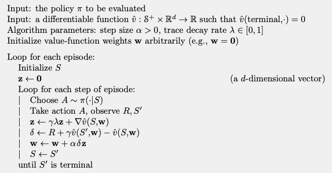
\[\mathbf{w}_{t+1} = \mathbf{w}_t + \alpha\delta_t\mathbf{z}_t\]We now have all the tools to write the algorithm:
Semi-gradient TD(\(\lambda\))
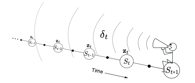
We can represent the update step has a backward update:
Each update depends on the current TD error.
Combined with the current eligibility traces of past events.
10.3. Sarsa(\(\lambda\))
Now we can modify Sarsa to work with the eligibility traces.
We want to learn the approximate action values \(\hat{q}(s,a,\mathbf{w})\).
The update of the weight vector is the same:
\[\mathbf{w}_{t+1} = \mathbf{w}_t + \alpha\delta_t\mathbf{z}_t\]The TD error changes, because it uses the q-value function and not the value function:
\[\delta_t = r_{t+1} + \gamma\hat{q}(s_{t+1},a_{t+1},\mathbf{w}_t) - \hat{q}(s_t,a_t,\mathbf{w}_t)\]Same thing for the eligibility trace:
The pseudocode of the algorithm is:
Sarsa(\(\lambda\))
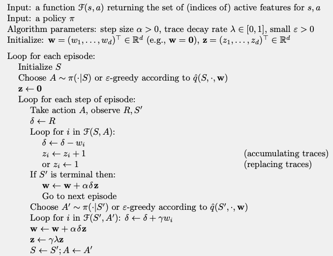
Activity
Read the pseudocode and try to understand it.