6. Dynamic Programming
We have seen in two previous topics how we can model a problem and how we can determine the best policy.
The only thing missing is an algorithm to calculate the optimal policy and value function.
There are different approaches:
Dynamic programming
Monte-Carlo methods
Reinforcement learning
Dynamic programming is the first proposed and it gives the foundations.
Activity
What do we need to calculate to obtain the optimal policies?
Give the formulas.
6.1. Policy Iteration
The algorithm works in two parts:
Policy evaluation (prediction)
Policy improvement
6.1.1. Policy Evaluation
The idea of policy evaluation is to compute the value function \(v_\pi\) for a policy \(\pi\).
Remember the equation from the previous topic:
It is possible to calculate this equation by iterative methods.
Consider a sequence of approximate value functions \(v_0, v_1, v_2, \dots\).
We initialize \(v_0\) with an initial value and the goal state to \(0\).
Each successive approximation is calculated as defined above:
\[v_{k+1}(s) = \sum_a\pi(a|s)\sum_{s'}p(s'|s,a)\left[ r(s,a) + \gamma v_k(s') \right]\]This update function will converge to \(v_\pi\) as \(k \rightarrow \infty\).
Of course at each step you need to calculate \(v_k(s)\) for every state \(s \in S\).
Put in an algorithm we obtain:
Algorithm
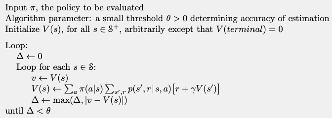
Example
We will consider the following problem, initial policy, and initial value function.
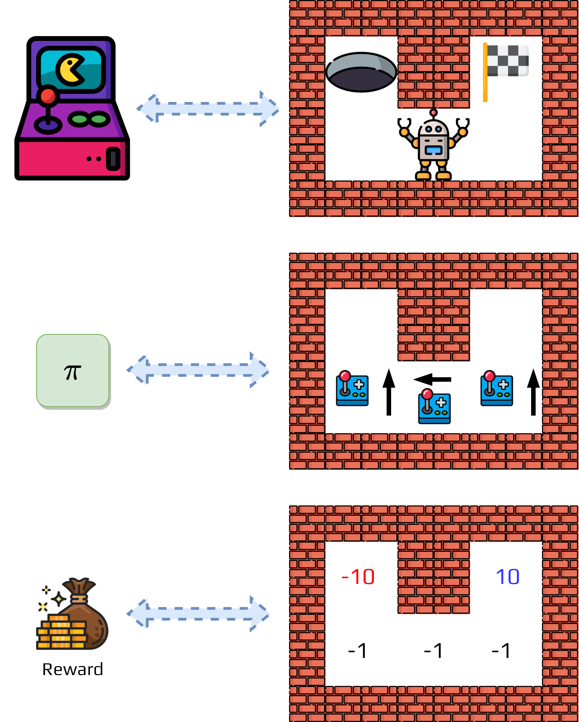
Now we estimate the value function using the formula.

6.1.2. Policy Improvement
Now we can evaluate a policy, it is possible to find a better one.
The idea is simple:
We take our value function \(v_\pi\).
We choose a state \(s\).
And we check if we need to change the policy for an action \(a, a\neq \pi(s)\).
A way to verify this is to calculate the q-value:
Then we can compare the value obtain with the one in the current value function.
Policy improvement theorem
Let \(\pi\) and \(\pi'\) being any pair of deterministic policies such that, for all \(s\in S\),
Then the policy \(\pi'\) must be as good as, or better than \(\pi\).
That is, it must obtain greater or equal expected return from all states \(s\in S\):
The intuition is that if, for a policy, we change only the action for a state \(s\), then the changed policy is indeed better.
Now, we just need to apply this to all states.
Each time we select the action that seems better according to \(q_\pi(s,a)\):
This greedy method respect the policy improvement theorem.
6.1.3. Policy Iteration Algorithm
The policy iteration algorithm combines the two previous steps.
It calculates the optimal policy by executing the previous steps multiple time:
Evaluate a policy
Improve the policy
If the policy changed go to step 1.
MDPs has a finite number of policies, so it will converge to the optimal policy.
The complete algorithm is:
Policy Iteration
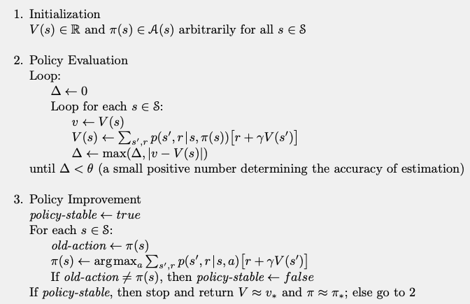
Example
Following the previous example, we can apply policy iteration.

Activity
Suggest possible drawback of this method.
6.2. Value Iteration
Considering the issue with Policy Iteration, we could come up with another algorithm.
It is possible to only consider a one-step policy evaluation.
This algorithm is Value Iteration.
It proposes to do only one step evaluation combined with policy improvement.
We obtain the following formula:
\[\begin{split}\begin{aligned} v_{k+1}(s) &= \max_a \mathbb{E}\left[ r_{t+1} + \gamma v_k(s_k) | s_t = s, a_t = a \right]\\ &= \max_a\sum_{s'}p(s'|s,a)\left[ r(s,a) + \gamma v_k(s') \right]\\ \end{aligned}\end{split}\]It updates the value function, but we lose our stopping criteria.
As it can take an infinite number of steps to converge to the optimal value function, we need to define when to stop.
In practice, we fix a small value, and when the value function change by less than this value we stop.
The complete algorithm is:
Value Iteration
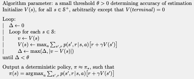
This algorithm converge faster than policy iterations.