3. Multi-armed bandit - Action Selection methods
In the previous topic we saw an algorithm to update the action-value.
The algorithm updates the action-value by averaging the rewards.
This method consider that every reward has the same weights.
Another popular way in reinforcement learning is to give more weights to the more recent rewards.
3.1. Constant step-size parameter
If we take the previous formula and we replace it with a constant parameter \(\alpha\) we obtain:
\[Q_{n+1} = Q_n + \alpha\left[ R_n - Q_n \right]\]where the step-size parameter \(\alpha \in (0,1]\) is constant.
\(Q_{n+1}\) is called a weighted average of post rewards and initial estimate \(Q_1\):
Note
It is called a weighted average because the sum of the weights is:
3.2. Action-value initialization
We have seen that the algorithm is initialized with some default action-value estimate \(Q_1(a)\).
This method is statistically biased by the initial estimate.
For the sampled average, the bias disappears once all actions have been selected.
However, for the weighted average, the bias is permanent. Even if it decreases over time.
Example
We can compare the sampled average and the weighted average.
We will initialize the weighted average of action 4 to something neutral like 0.
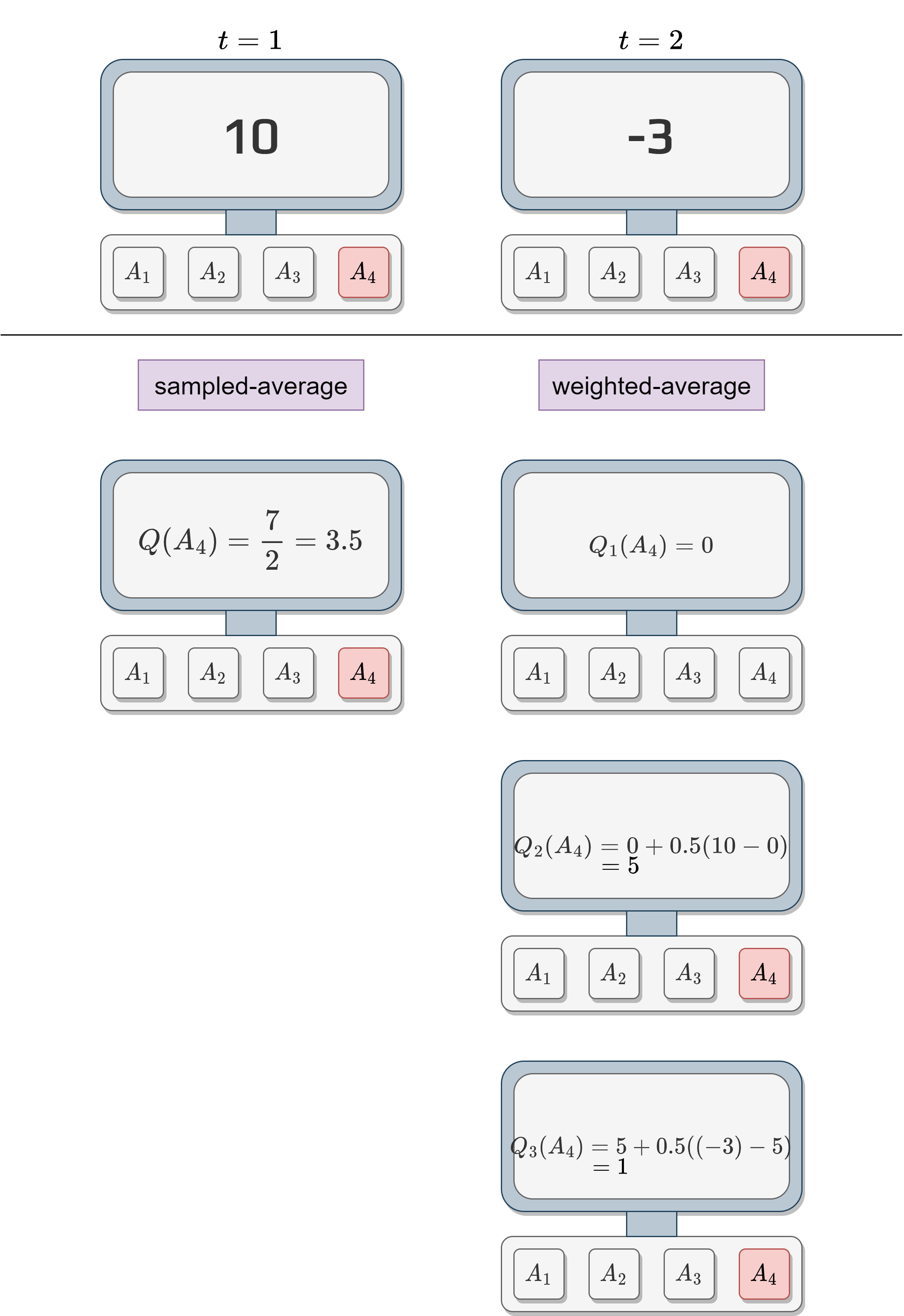
We can see that the sampled-average value and the weighted average value are not the same.
This bias cannot be overcome by choosing different initial value.
Setting all the actions to a positive value is optimistic.
After trying one action:
The algorithm will be disappointed by the returned reward (compared to the estimate).
It will select another action due to this disappointment.
Because all the actions are over optimistic, the algorithm will choose all of them multiple times.
3.3. Upper-Confidence-Bound action-selection
Let’s think about the action-selection seen until now.
Greedy action-selection:
Always choose the action that has the higher expected reward.
It doesn’t explore.
\(\epsilon\)-greedy action-selection:
It forces the selection of non-greedy action based on a probability \(\epsilon\).
No preferences between non-greedy action.
Activity
What is the downfall of \(\epsilon\)-greedy?
It is possible to improve the action-selection by adding a few parameters to the selection algorithm.
The idea is to base the exploration on the uncertainty of the estimate.
Having a high uncertainty means that we didn’t explore the action often compared to the numbers of action selected in total.
If we don’t have a good estimate, we should explore.
We call this Upper-Confidence bound.
The action-selection formula becomes:
\[A_t = \arg \max_a\left[ Q_t(a)+c\sqrt{\frac{\ln t}{N_t(a)}} \right]\]where
\(\ln t\) is the natural logarithm of \(t\),
\(N_t(a)\) is the number of time \(a\) has been selected,
and \(c>0\) the degree of exploration.
Activity
What happens when \(N_t(a)\) increase?
What happens when \(\ln t\) increase?
When our uncertainty on the estimate decrease the action is less selected.
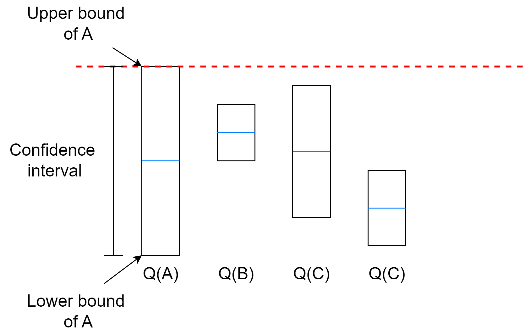
The algorithm will select the action with the highest upper bound even if the uncertainty is very high.
If multiple actions have very close upper bounds, it will depend on the exploration coefficient.
Activity
If we use our previous samples.
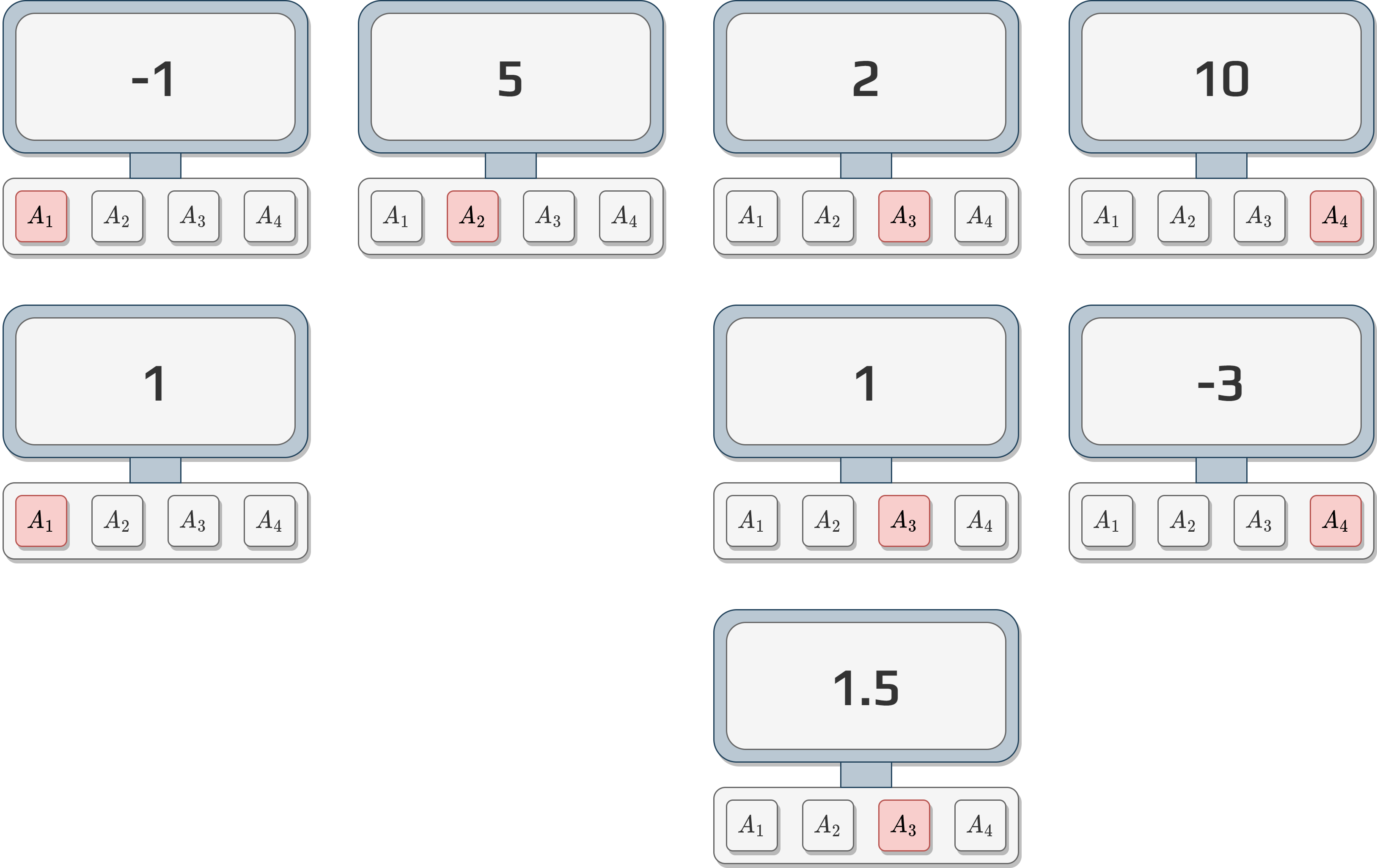
Calculate each \(Q\) values using the weighted average.
Use UCB with \(c=2\) to decide what will be the next action.
3.4. Gradient Bandit Algorithms
All previous methods have one thing in common.
They all based the action-selection on received rewards.
We will discuss another technic based on the preference of an action \(a\), \(H_t(a)\).
Higher the preference is, more often the action is selected.
We use this preference in a softmax distribution:
\[P(A_t=a)=\frac{e^{H_t(a)}}{\sum_{b=1}^{k}e^{H_t(b)}}=\pi_t(a)\]where \(\pi_t(a)\) is the probability to select \(a\) at time \(t\).
Now, we need to calculate the preference \(H_t(a)\).
At the beginning \(H_1(a) =0, \forall a \in A\).
We use stochastic gradient ascent.
After each action \(A_t\) the preference is updated:
\[\begin{split}\begin{aligned} H_{t+1}(A_t) &= H_t(A_t) + \alpha(R_t - \bar{R}_t)(1-\pi_t(A_t))\text{, and}\\ H_{t+1}(a) &= H_t(a) - \alpha(R_t - \bar{R}_t)\pi_t(a)\text{, for all } a \neq A_t \end{aligned}\end{split}\]where \(\alpha >0\) is the step-size parameter, \(\bar{R}_t \in \mathbb{R}\) is the average reward not including time \(t\).
We often refer to \(\bar{R}_t\) as the baseline.
Activity
What happens if the reward is greater than the baseline?
What happens if the reward is less than the baseline?