9. Approximation - On-Policy
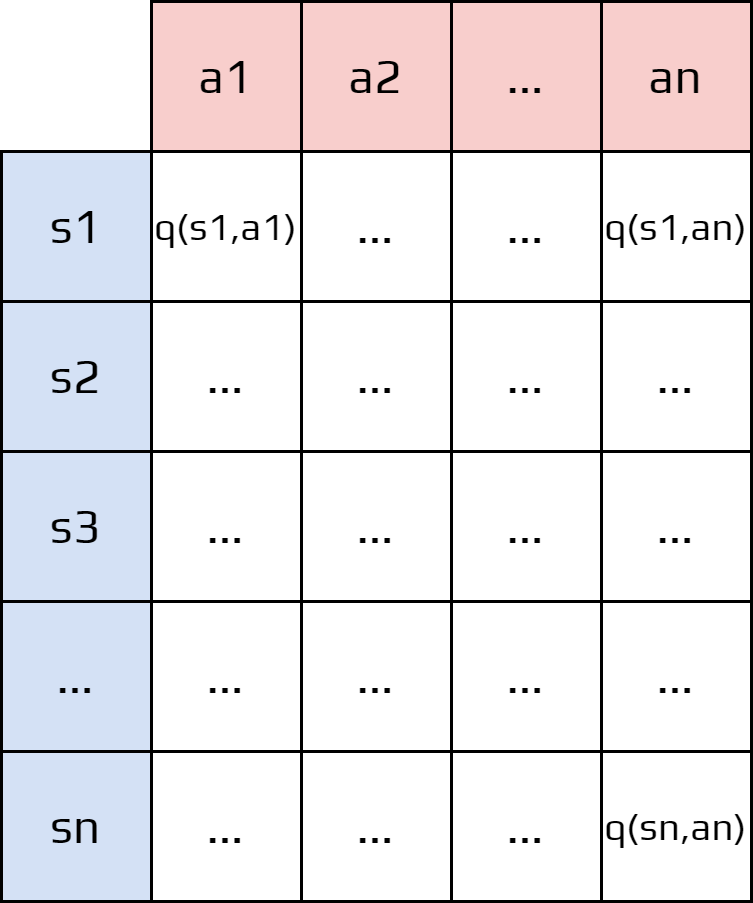
The methods seen until now were Tabular Methods.
For each pair state-action, we estimate the value \(q_\pi(s,a)\).
Basically, we create a big table.
Activity
What is the issues with this type of method?
The only solution is to aim for a good approximation.
9.1. Value-Function Approximation
To avoid using a table, we will use a weight vector \(\mathbf{w}\in \mathbb{R}^d\).
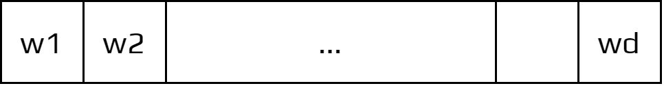
The approximate value of state \(s\) will be written as \(\hat{v}(s,\mathbf{w})\).
The vector \(\mathbf{w}\) is for every state, so we don’t calculate one per state!
The dimension of the \(\mathbf{w}\) is less than the number of states ( \(d \ll |S|\)).
Important
The weight vector is how we reduce the complexity.
We need to come back on certain terms and notations:
During the update we shifted the value of \(v(s)\) to the update target.
We refer to an individual update by the notation \(s \mapsto u\).
\(s\): the state
\(u\): the update target
For MC methods: \(s_t \mapsto G_t\).
For TD(0): \(s_t \mapsto r_{t+1} + \gamma\hat{v}(s_{t+1})\)
It signifies that you move the previous value slightly to the new one.
With a weight vector we can have more complex functions to update the value function.
Note
The weight vector is now calculated using deep neural networks.
9.2. Prediction Objective
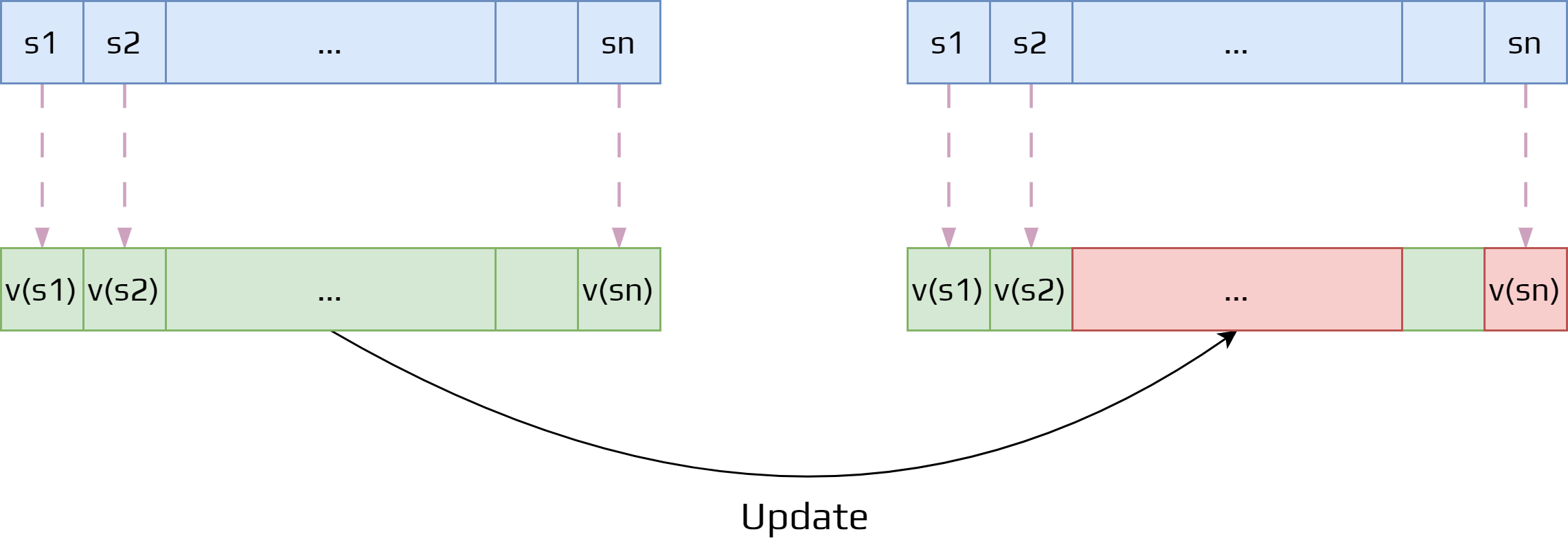
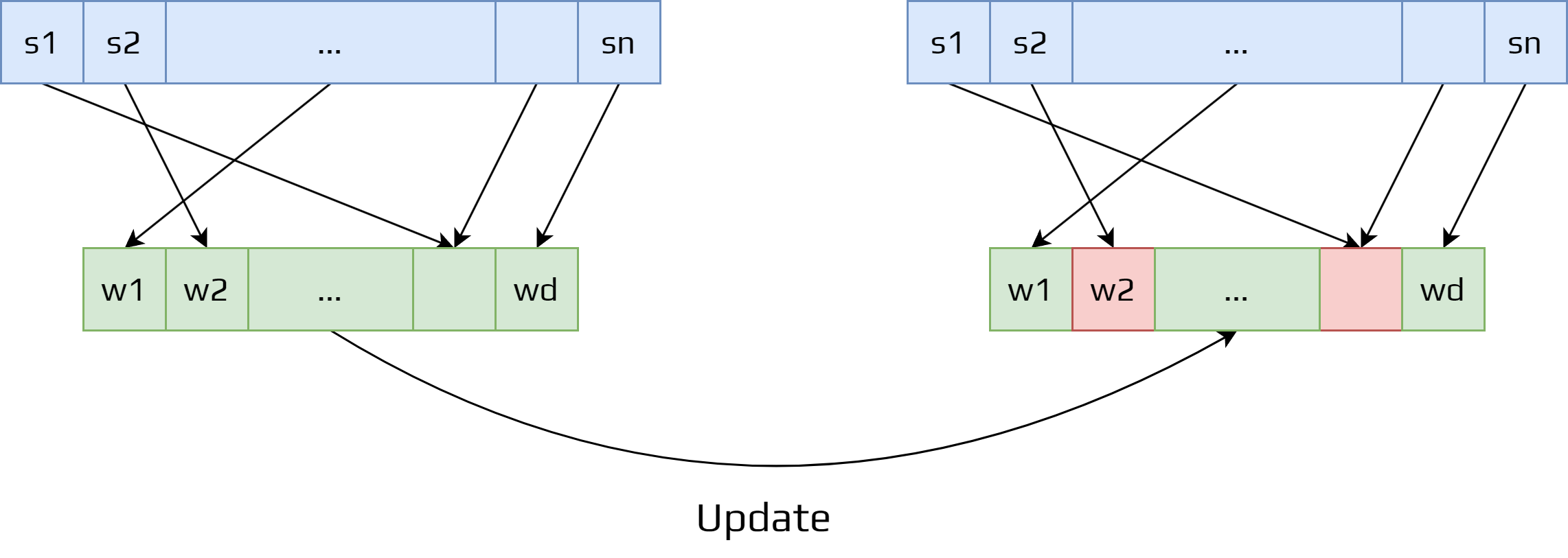
However, having a weight vector smaller than the number of states have certain issues.
An update done at one state affects other states.
As it is an approximation, it is not possible to get the values of all states.
So making one state’s estimate more accurate invariably means making others’ less accurate.
To solve this issue, we need to specify which states are more important.
We create a state distribution: \(\mu (s)\geq 0, \sum_s\mu (s)=1\).
States with higher value are more important.
The idea is to reduce the error for these states.
The difference between the estimated value \(\hat{v}(s,\mathbf{w})\) and the true value \(v_\pi(s)\).
The function is called the mean square value error and is defined as:
\[\overline{\text{VE}}(\mathbf{w}) = \sum_{s\in S}\mu (s)\left[ v_\pi(s) - \hat{v}(s,\mathbf{w}) \right]^2\]Often \(\mu (s)\) is chosen to be a fraction of the time spent in the state \(s\).
This method is called on-policy distribution.
Important
It is not guaranteed that \(\overline{\text{VE}}\) will lead to the global optimum.
Usually it converges to a local optimum.
9.3. Stochastic-gradient Methods
It is now time to see in detail the most important class of learning methods for function approximation.
The stochastic gradient descent (SGD).
9.3.1. Gradient Descent
Gradient descent algorithm is used to find a local minimum (or maximum) of a function.
As we will see it is very popular in Reinforcement Leaning and Deep Learning.
Important
The main requirement is that the function needs to be differentiable. Meaning that the function has a derivative for each point in its domain.
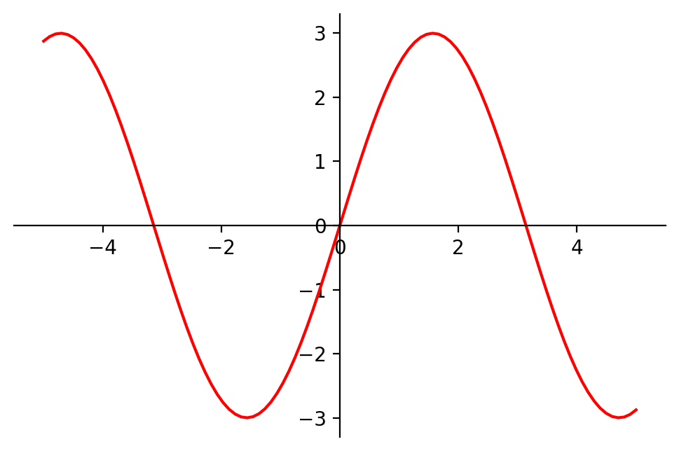
A gradient is a slope of a curve at a given point in a specified direction.
In the case of a univariate function, it is simply the first derivative at a selected point.
In the case of a multivariate function, it is a vector of derivatives in each main direction (along variable axes).
Because we are interested only in a slope along one axis (and we don’t care about others) these derivatives are called partial derivatives.
So a gradient for an \(n\)-dimensional function \(f(x)\) at a given point \(p\) is defined as follows:
Example
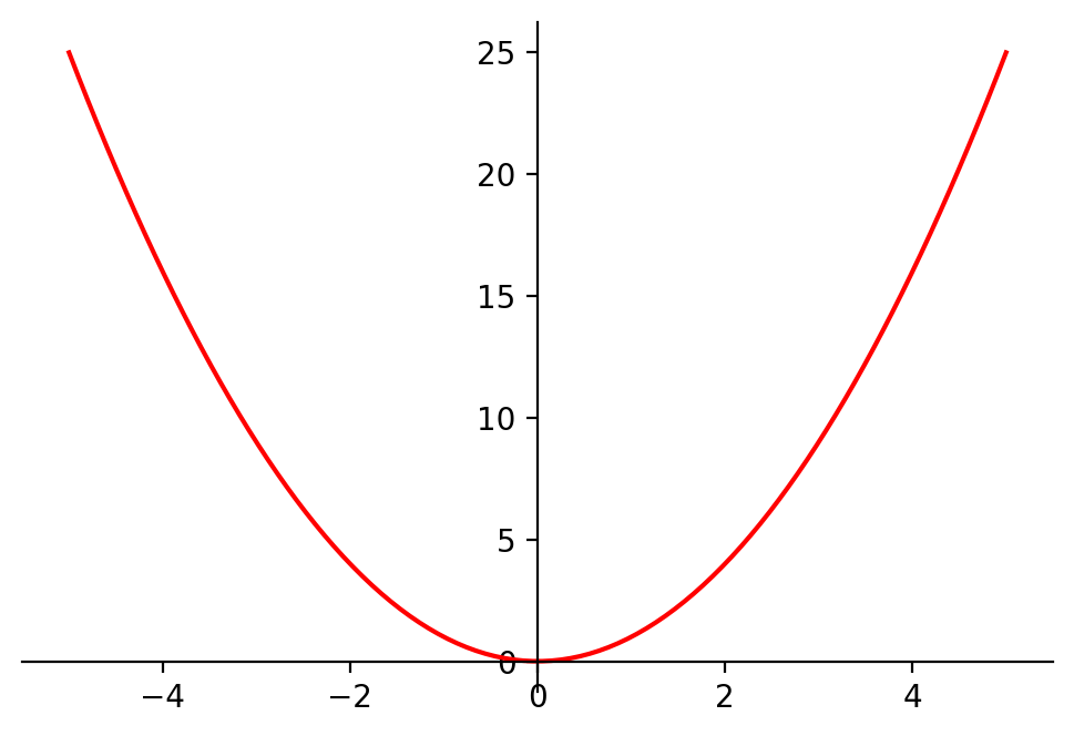
Consider a function \(f(x,y) = 0.5 x^2 + y^2\).
Then \(\nabla f(x,y) = \begin{bmatrix}\frac{\partial f(x,y)}{\partial x} \\\frac{\partial f(x,y)}{\partial y} \end{bmatrix} = \begin{bmatrix}x\\ 2y \end{bmatrix}\).
Now if we take \(x = 10\) and \(y = 10\), we obtain \(\nabla f(10,10) = \begin{bmatrix}10\\ 20 \end{bmatrix}\)
The gradient descent algorithm just calculates iteratively the next point using:
\[p_{n+1} = p_{n} - \eta\nabla f(p_n)\]\(\eta\) being the learning rate.
The algorithm stop when the step size \(\eta\nabla f(p_n)\) is les than a tolerance.
It can be implemented very easily in python:
import numpy as np

def gradient_descent(start, gradient, learn_rate, max_iter, tol=0.01):
   steps = [start] # history tracking
   x = start

   for _ in range(max_iter):
      diff = learn_rate*gradient(x)
      if np.abs(diff)<tol:
         break
      x = x - diff
      steps.append(x) # history tracing

   return steps, x
Activity
Calculate gradient function of \(f(x) = x^2 - 4x + 1\).
Execute three steps of the gradient descent algorithm starting with \(x=9\) and \(\eta=0.1\).
9.3.2. Stochastic-Gradient methods in RL
In gradient-descent methods:
The weight vector is a column vector \(\mathbf{w} = (w_1, w_2,\dots,w_d)^\intercal\).
The approximate value function \(\hat{v}(s,\mathbf{w})\) is a differentiable function of \(\mathbf{w}\) for all \(s\in S\).
To see how it works, we will assume a few things:
At each step we observe \(s_t \mapsto v_\pi(s_t)\), a state and its true value under \(\pi\).
States appear with the same distribution \(\mu\) we are trying to minimize the \(\overline{\text{VE}}\):
\[\overline{\text{VE}}(\mathbf{w}) = \sum_{s\in S}\mu (s)\left[ v_\pi(s) - \hat{v}(s,\mathbf{w}) \right]^2\]We could try to do it on the sample observed.
That is what SGD is doing:
\[\begin{split}\begin{aligned} \mathbf{w}_{t+1} &= \mathbf{w}_t - \frac{1}{2}\alpha\nabla\left[ v_\pi(s_t) -\hat{v}(s_t,\mathbf{w}_t) \right]^2\\ &= \mathbf{w}_t + \alpha\left[ v_\pi(s_t) - \hat{v}(s_t,\mathbf{w}_t) \right]\nabla\hat{v}(s_t,\mathbf{w}) \end{aligned}\end{split}\]where \(\alpha\) is a positive step-size, and \(\nabla f(\mathbf{w})\) denotes the vector of partial derivatives:
\[\nabla f(\mathbf{w}) = \left( \frac{\partial f(\mathbf{w})}{\partial w_1},\dots, \frac{\partial f(\mathbf{w})}{\partial w_d} \right)^T\]A few precision:
It is called a gradient descent method, because the step in \(\mathbf{w}_t\) is proportional to the negative gradient of the squared error.
It is said stochastic when it’s done on a single state that is chosen stochastically.
9.3.3. Estimating the weight vector
Usually, we don’t observe the true value of a state \(v_\pi (s)\).
In general, we have a approximate value \(U_t\) at time \(t\).
If \(U_t\) is an unbiased estimate, then we can rewrite the previous equation:
Example
Now if we consider a Monte-Carlo approach.
We don’t observe the true value of a state but we simulate interaction with the environment.
It gives an expected return \(G_t\).
This returned is unbiased, so we can say that \(U_t = G_t\).
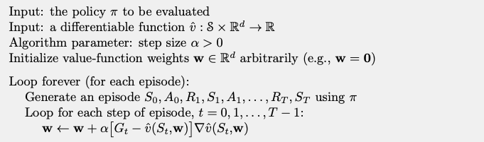
Letting us apply the gradient descent:
Gradient descent for Monte-Carlo
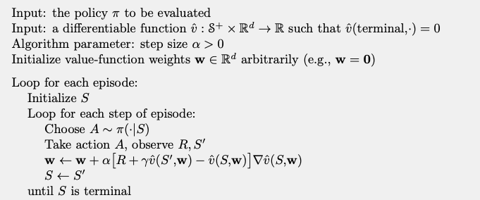
Now, we need to consider what happens for bootstrapping methods.
Remember TD(0) is a bootstrapping algorithm.
Bootstrapping methods are not a true gradient descent.
They take into account the effect of changing the weight vector \(\mathbf{w}_t\) on the estimate,
but ignore its effect on the target.
Consequently, it is called semi-gradient methods.
It converges to the local optimal, but not as fast.
In the case of TD(0), we have \(U_t = r_{t+1} + \gamma\hat{v}(s_{t+1},\mathbf{w})\) as the target.
The pseudocode of the algorithm is given below:
Semi-gradient TD(0)
9.4. On-policy Control
Until now, we saw how to estimate the error function based on a given policy \(\pi\)
To take into account the vector of weight \(\mathbf{w}\) we can rewrite of q-function from \(q^*(s,a)\) to \(\hat{q}(s,a,\mathbf{w})\).
We will extend TD(0) to on-policy control.
The new algorithm is called Sarsa.
The main difference with policy estimation is that use \(\mathbf{w}\) for the q-function.
The gradient-descent update for action-value is defined as:
\[\mathbf{w}_{t+1} = \mathbf{w}_t + \alpha\left[ U_t - \hat{q}(s_t,a_t,\mathbf{w}_t) \right] \nabla\hat{q}(s_t,a_t,\mathbf{w}_t)\]where \(U_t\) can be any approximation of \(q_\pi(s_t,a_t)\).
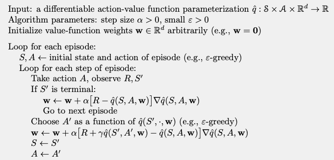
In our case, we are interested in the one-step Sarsa algorithm, so we can rewrite it as:
\[\mathbf{w}_{t+1} = \mathbf{w}_t + \alpha\left[ r_t + \gamma\hat{q}(s_{t+1}, a_{t+1}, \mathbf{w}_t) - \hat{q}(s_t,a_t,\mathbf{w}_t) \right] \nabla\hat{q}(s_t,a_t,\mathbf{w}_t)\]This method is the episodic semi-gradient one-step Sarsa.
The idea for the algorithm is simple:
For each possible action \(a\), compute \(\hat{q}(s_{t+1}, a, \mathbf{w}_t)\).
Find the greedy action \(a^*_{t+1}=\arg\max_a\hat{q}(s_{t+1}, a, \mathbf{w}_t)\).
The policy improvement is done by changing the estimation policy to a soft approximation of the greedy policy such as \(\epsilon\)-greedy policy.
The pseudocode of the algorithm can be written as:
Semi-gradient Sarsa
9.5. Function Approximation
If you remember, we said that \(\mathbf{w}\in \mathbb{R}^d\) of dimension smaller that the number of states.
So it means that we don’t have a direct mapping fron \((s,a)\mapsto q_\pi(s,a)\).
We need a function approximation.
There are multiple types of approximation that we can use:
State-aggregation
Linear function
Neural networks
Etc.
9.5.1. State-aggregation
It is the simplest one.
You split the states in groups that should be similar enough.
Then the value function will asign the same value for the states in the same group.
Works for very simple problems.
9.5.2. Linear Function
One of the most important special cases of function approximation.
The approximate function \(\hat{v}(.,\mathbf{w})\) is a linear function of \(\mathbf{w}\).
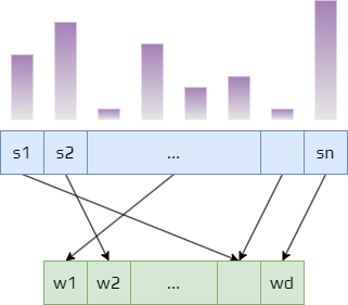
To every state \(s\), there is a real-valued vector \(\mathbf{x}(s) = (x_1(s0), x_2(s),\dots, x_d(s))^T\).
Linear methods approximate the state-value function by the inner product between \(\mathbf{w}\) and \(\mathbf{x}(s)\):
The vector \(\mathbf{x}(s)\) is called a feature vector representing state \(s\).
It is interesting in stochastic gradient descent, because the gradient is simply:
Thus the update in the linear case, just becomes:
9.5.3. Feature Construction for Linear Methods
Linear methods are powerful and efficient, but they depends mainly on how the states are represented in terms of features.
A limitation of the linear form is that it cannot take into account any interactions between features.
Activity
Give some examples of problems where we would like to know the interaction of two features.
We would need the combination of these two fetures in another feature.
Polynomial functions are a simple way to do that.
Example
Suppose a reinforcement learning problem has states with two numerical dimensions.
A state will be represented by two values: \(s_1\in \mathbb{R}\) and \(s_2\in \mathbb{R}\).
You could be tempted to use a 2D feature vector \(\mathbf{x}(s) = [s_1, s_2]^T\).
With this representation the interaction between \(s_1\) and \(s_2\) cannot be represented.
Also, if \(s_1 = s_2 = 0\), the the approximation would always be 0.
It can be solved by adding some features: \(\mathbf{x}(s) = [1, s_1, s_2, s_1s_2]^T\)
Or even add more dimensions: \(\mathbf{x}(s) = [1, s_1, s_2, s_1s_2, s_1^2,s_2^2,s_1^2s_2,s_1s_2^2,s_1^2s_2^2]^T\).