11. Policy Gradient Methods
Until now, we used action-value methods.
The action selected in a state depends of its estimated value.
In this topic, we will see another method.
Instead of learning an action value function, we will learn a parameterized policy that can select actions without a value function.
Note
A value function can be used to learn the policy, but is not necessary.
We define \(\mathbf{\theta} \in \mathbb{R}^{d'}\) the policy parameter vector.
The probability that an action \(a\) is taken at time \(t\) in state \(s\) and parameter \(\mathbf{\theta}\) is defined as:
\[\pi(a|s,\mathbf{\theta}) = P(a_t = a|s_t = s,\mathbf{\theta}_t = \mathbf{\theta})\]Again the policy parameter will be learned using a gradient of a scalar performance measure \(J(\mathbf{\theta})\).
In this case we want to maximize the performance, so the update is a gradient ascent in \(J\):
\[\mathbf{\theta}_{t+1} = \mathbf{\theta}_{t} + \alpha\widehat{\nabla J(\mathbf{\theta}_t)}\]where \(\widehat{\nabla J(\mathbf{\theta}_t)} \in \mathbb{R}^{d'}\) is a stochastic estimate whose expectation approximates of the performance measure with respect to its argument \(\mathbf{\theta}_t\).
11.1. Policy Approximation and its Advantages
In policy gradient methods, the policy can be parameterized in any way.
The only condition is that \(\pi(a|s,\mathbf{\theta})\) is differentiable with respect to its parameters.
In practice we require that the policy never becomes deterministic.
Activity
Why don’t we want to have a deterministic policy in policy gradient methods?
If the action space is discrete and not too large:
We could create a parameterized numerical preference \(h(s, a, \mathbf{\theta})\in \mathbb{R}\) for each state-action pair.
The actions with the highest preferences in each state are given the highest probabilities of being selected.
It can be done with a softmax distribution:
\[\pi(a|s,\mathbf{\theta}) = \frac{e^{h(s,a,\mathbf{\theta})}}{\sum_b e^{h(s,b,\mathbf{\theta})}}\]Parameterizing policies according to softmax has two advantages:
The approximate policy can approach a deterministic policy, whereas with \(\epsilon\)-greedy will always have a probability to choose a suboptimal action.
It enables the selection of actions with arbitrary probabilities. Some problem doesn’t have one optimal action for a state, but multiple with different probabilities.
11.2. REINFORCE: Monte Carlo Policy Gradient
Our first policy gradient algorithm is based on Monte Carlo.
It is always an easy algorithm to implement.
The policy gradient theorem give establishes:
It provides an analytic expression for the gradient of performance with respect to the policy parameter.
It does not involve the derivative of the states distribution.
Note
We will not see the proof, but you can look it up if you’re interested.
If we stop there, we could create our gradient-ascent algorithm as:
where \(\hat{q}\) is some learned approximation to \(q_\pi\).
However, we want to modify REINFORCE.
So, we introduce an action \(a\) by replacing a sum over the random variable’s possible values by an expectation under \(\pi\).
The previous equation does not have the term weighted by \(\pi(a|s,\mathbf{\theta})\).
We can change that by multiplying and then dividing the summed terms by \(\pi(a|s,\mathbf{\theta})\):
The final expression is a quantity that can be sampled.
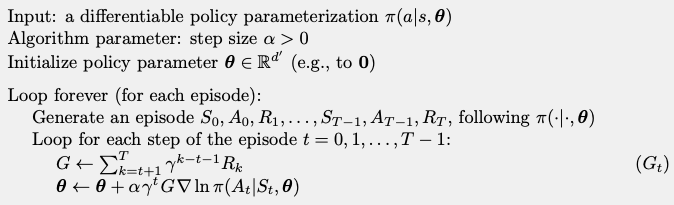
If we integrate that to our algorithm, we have the following update of the parameters:
Concretly:
Each increment is proportional to the product of a return \(G_t\) and a vector.
The vector is the direction in parameter space that most increases the probability of repeating the action \(a_t\) on future visits to state \(s_t\).
The update increases the parameter vector in this direction proportional to the return, and inversely proportional to the action probability.
The former makes sense because it causes the parameter to move most in the directions that favour actions that yield the highest return.
The latter makes sense because otherwise actions that are frequently selected are at an advantage and might win out even if they do not yield the highest return.
The pseudocode of the algorithm is written as:
Mote Carlo policy-gradient
11.3. Actor-Critic methods
We have seen with TD and SARSA that a one-step update is often more interesting in terms of computation.
However, the previous policy-gradient method requires the entire return.
Actor-critic methods allow us to have a one-step policy gradient.
The idea:
We use the q-value to assess the action.
When q-values are used this way it is called a critic.
And the policy is an actor.
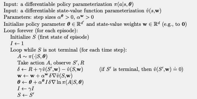
We replace the full return of REINFORCE by a one-step return as follows:
\[\begin{split}\begin{aligned} \mathbf{\theta}_{t+1} &= \mathbf{\theta}_t + \alpha\left( G_{t:t+1}-\hat{v}(s_t,\mathbf{w}_t) \right)\frac{\nabla\pi (a_t|s_t,\mathbf{\theta}_t)}{\pi (a_t|s_t,\mathbf{\theta}_t)}\\ &= \mathbf{\theta}_t + \alpha\left( r_{t+1} + \gamma\hat{v}(s_{t+1},\mathbf{w}) -\hat{v}(s_t,\mathbf{w}) \right)\frac{\nabla\pi (a_t|s_t,\mathbf{\theta}_t)}{\pi (a_t|s_t,\mathbf{\theta}_t)}\\ &= \mathbf{\theta}_t + \alpha\delta_t\frac{\nabla\pi (a_t|s_t,\mathbf{\theta}_t)}{\pi (a_t|s_t,\mathbf{\theta}_t)}\\ \end{aligned}\end{split}\]It is combined with the state-value-function of TD(0) and we obtain the following algorithm:
One-step Actor-critic
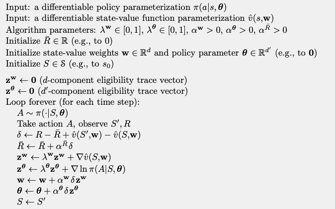
Of course, we can use the eligibility trace if we want:
Eligibility traces Actor-critic
11.4. Continuous Actions
Some problems can have continuous actions.
Until now the previous methods were suing q-values, thus tabular methods.
It would be very complicated to adapt this types of methods to continuous actions.
Thankfully, policy-gradient offers a very practical way to do that!
Activity
Give some problems that have very large or continuous action space?
How does it work:
We don’t compute the probability for each action.
We learn a probability distribution.
We could choose to use a Gaussian distribution to select the actions:
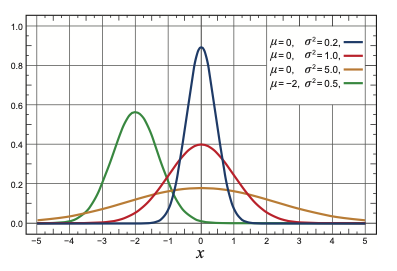
If we want to use a normal distribution with a policy parameterization, then we can rewrite \(\pi(a|s,\mathbf{\pi})\) as a normal distribution:
It also implies that the policy’s parameter vector is in two parts, \(\mathbf{\theta}=[\mathbf{\theta}_\mu, \mathbf{\theta}_\sigma]^T\).