5. Policies and Value Function
In the previous topic, we introduced formally Markov Decision Processes.
The objectives of MDP is to maximize the cumulative reward.
We will see how it can be done and how it is linked to the action selection.
5.1. Cumulative rewards
Remember that after few times steps we obtain a trajectory:

Similarly we also obtain a sequence of rewards associated to this trajectory:

As the objective is to maximize the cumulative rewards, we need to consider which part of this sequence we want to maximize.
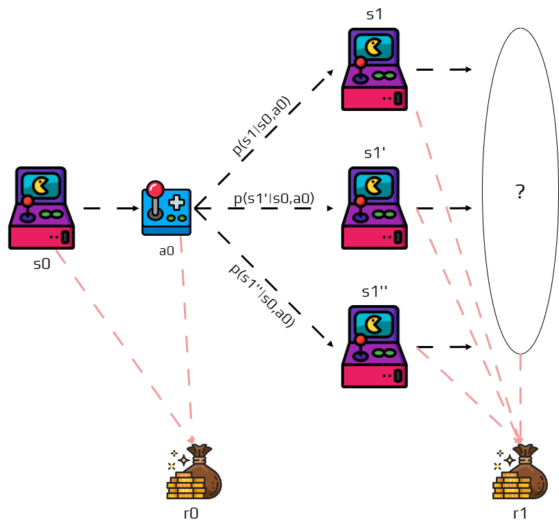
Remember that for a same action in a same state the next future state is not certain, so it complicates things.
This is why, in reinforcement learning we try to maximize the expected return.
The return is denoted \(G_t\) and can be defined as the sum of the rewards:
\[G_t = r_{t}, r_{t+1}, \dots, r_T\]where \(T\) is the final step.
As you can see it is very well defined when \(T\) has a maximum value.
Example
You receive three times a reward of \(10\).
\(G_t\) is the sum of thiss rewards, so \(30\).

Activity
What happens if \(T=\infty\), meaning if the problem does not end?
Due to this issue, it was introduced the notion of discounted return:
\[G_t = r_{t} + \gamma r_{t+1} + \gamma^2 r_{t+2} = \sum_{k=0}^\infty \gamma^k r_{t+k}\]where \(\gamma\) is a parameter \(0\leq\gamma\leq 1\) called discount rate.
This discount rate represents how much future rewards are important compared to immediate rewards.
A reward received at step \(k\) is worth only \(\gamma^k\) times what it would be worth now.
If \(\gamma = 0\) the agent only consider immediate reward, thus is greedy.
When \(\gamma\) approaches \(1\), the agent becomes farsighted.
Example
You receive three times a reward of \(10\).
But you apply a discount rate \(\gamma = 0.5\).

Important
If \(\gamma < 1\) has a finite value if the sequence is bounded.
This is crucial part of reinforcement learning.
It works well, because the returns at each time step are related to each other:
Note
Even if \(T=\infty\) the return is still finite
if the reward is nonzero and constant and,
if \(\gamma < 1\)
For example, is the reward is a constant \(+1\), then the return is:
5.2. Policies and Value functions
We know how to calculate the expected return of a sequence of rewards.
Now, we need to link that to our trajectory and more precisely on the decision-making.
The agent is supposed to learn which action to take depending on the state.
To do that reinforcement learning algorithms implement a value function.
Estimates the expected return of being in a specific state.
Value functions are closely linked to policies.
Definition: Policy
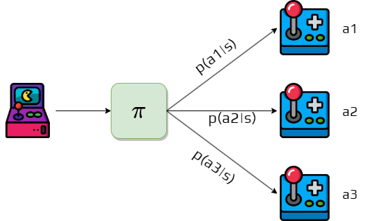
A policy is a mapping from states to probabilities of each possible action.
We denote a policy \(\pi\).
The probability that the agent following a policy \(\pi\) select an action \(a\) in state \(s\) is denoted \(\pi(a|s)\).
Definition: Value function
The value function of a state \(s\) under a policy \(\pi\) is the expected return when starting in \(s\) and following \(\pi\) thereafter.
In MDPs, \(v_\pi\) is defined as:
\[v_\pi(s) = \mathbb{E}_\pi\left[G_t | s_t=s \right] = \mathbb{E}_\pi\left[ \sum_{k=0}^\infty\gamma^k r_{t+k+1} | s_t = s \right]\]Note, that we used only the definition of \(G_t\).
Now we can estimate the value of a state.
However, we need to estimate the value of a specific action in a state.
This is defined by q-values:
\[q_\pi(s,a) = \mathbb{E}_\pi\left[G_t | s_t=s , a_t = a\right] = \mathbb{E}_\pi\left[ \sum_{k=0}^\infty\gamma^k r_{t+k+1} | s_t = s, a_t = a \right]\]
Lastly, value functions are also recursive:
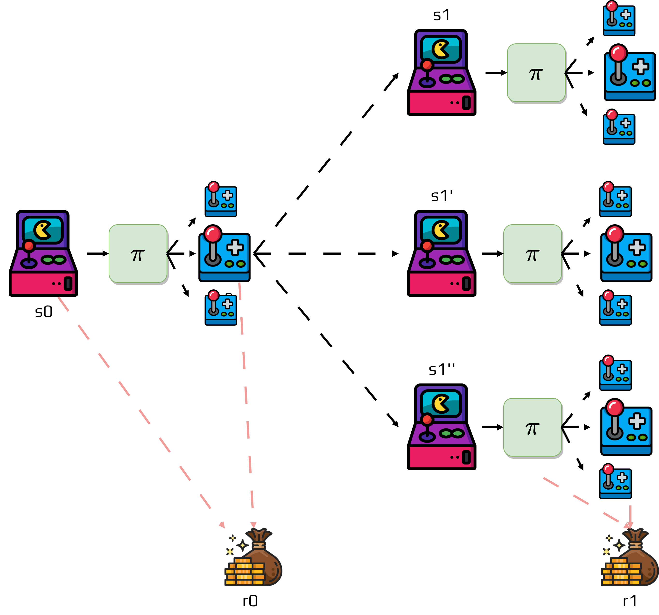
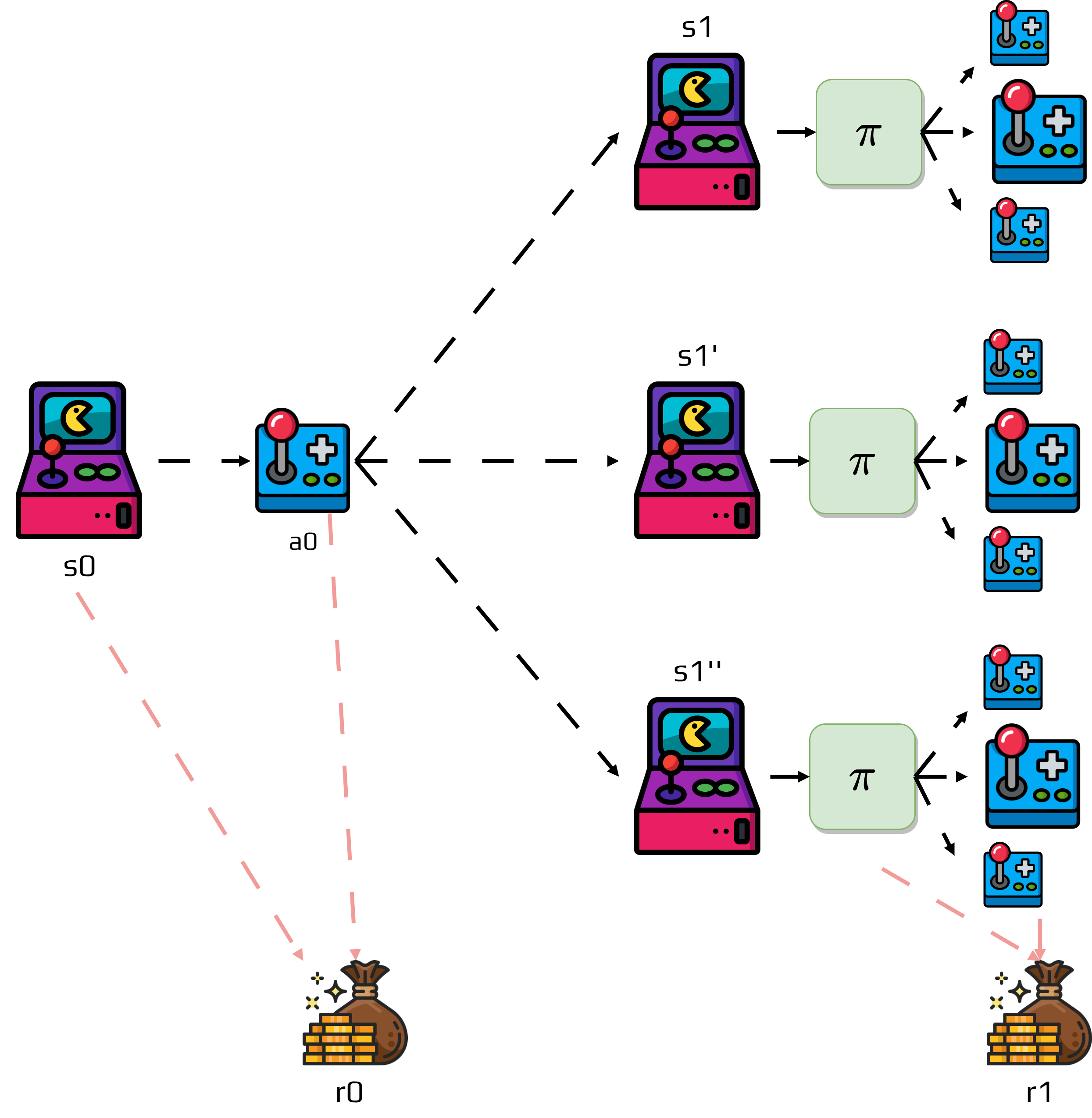
\[\begin{split}\begin{aligned} v_\pi(s) &= \mathbb{E}_\pi\left[G_t | s_t=s \right]\\ &= \mathbb{E}_\pi\left[r_{t} + \gamma G_{t}| s_t = s\right]\\ &= \sum_a \pi(a|s)\sum_{s'}p(s'|s,a)\left[ r(s,a) + \gamma\mathbb{E}_\pi\left[G_{t+1} | s_{t+1}=s' \right] \right]\\ &= \sum_a \pi(a|s)\sum_{s'}p(s'|s,a)\left[r + \gamma v_\pi(s')\right]\\ \end{aligned}\end{split}\]This is the Bellman equation applied to \(v_t\).
Remember your course on dynamic programming.
5.3. Optimal Policies and Optimal Value Functions
A policy \(\pi\) is just a mapping function.
Calculating a policy doesn’t guarantee that it’s optimal to solve the problem.
Activity
Propose a method to calculate the optimal policy.
Intuitively, we would like to compare two policies \(\pi, \pi'\) and find the best.
Concretely we want to create an ordering \(\pi > \pi'\).
Remember that a policy \(\pi\) has an associated value function \(v_\pi\).
We can compare policies by checking the return for each state \(s \in S\).
The policy is considered better if \(\forall s\in S, \pi(s)\geq\pi'(s)\).
Important
There is always at least one policy that is better than or equal to all other policies.
The optimal policy is denoted \(\pi^*\).
The optimal policy has an associated optimal value function.
The optimal value function is denoted \(v^*\) and defined as:
Activity
Discuss if for the same MDP we can find more than one optimal policy.
Because there is an optimal value function, there is an optimal q-value function:
We can rewrite the optimal value function as a Bellman equation:
Activity
What can you conclude from this equation?
To calculate the optimal policy, we “just” need to calculate the optimal value function.