2. Multi-armed bandit

• Remember the difference between reinforcement learning and unsupervised learning.

• Reinforcement learning uses training information to evaluate the actions.

• To really understand the RL we need to understand its evaluative aspect.

• We will consider the \(k\)-armed bandit problem.

2.1. What is the k-armed bandit problem?

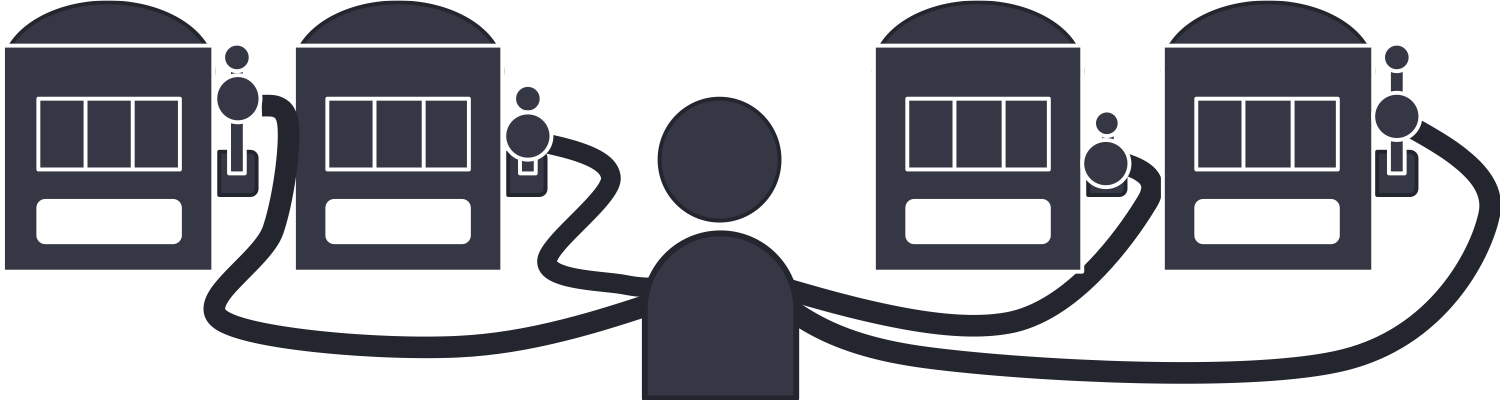
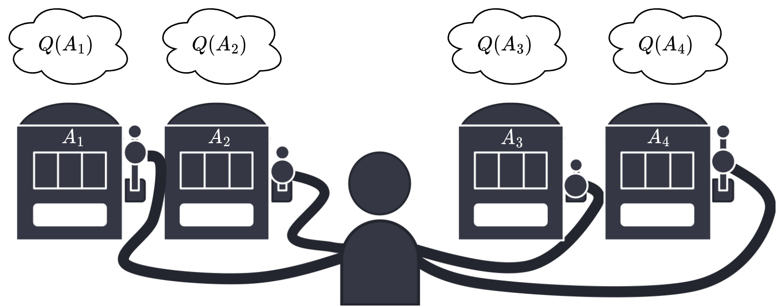
• An agent has \(k\) different actions.

• After taking an action, the agent receive a reward.

• The rewards are chosen from a stationary probability distribution based on the action selected.

• The objective of the agent is to maximize the expected total reward.

Activity

• Explain why the probability distributions are stationary.

• Why do we say expected total reward?

• More formally, each action has a value.

• We denote the action selected on a time step \(t\) as \(A_t\).

• We denote the corresponding reward as \(R_t\).

• We denote \(q_*(a)\) the expected reward of action \(a\):

\[q_*(a) = \mathbb{E}\left[ R_t|A_t=a \right]\]

• However, the estimated value of \(a\) at time \(t\) is denoted \(Q_t(a)\).

Activity

• Why do we have an estimated value?

• When you have \(Q_t(a)\) for all the actions:

  • Choosing \(a\) maximizing the reward is called greedy action selection.

    • It’s called exploitation.

    • It does not lead to the best expected value.

  • Choosing another action is called exploration.

    • It is necessary to update the estimations.

• We will see how we can balance exploration and exploitation.

2.2. Action-value methods

• Now, we need to estimate the actions.

• Then using these estimates to select the next action.

• The methods to do that are called action-value methods.

2.2.1. Estimating values

Activity

• Consider the following multi-armed bandit problem.

• Let us simulate a few actions and results:

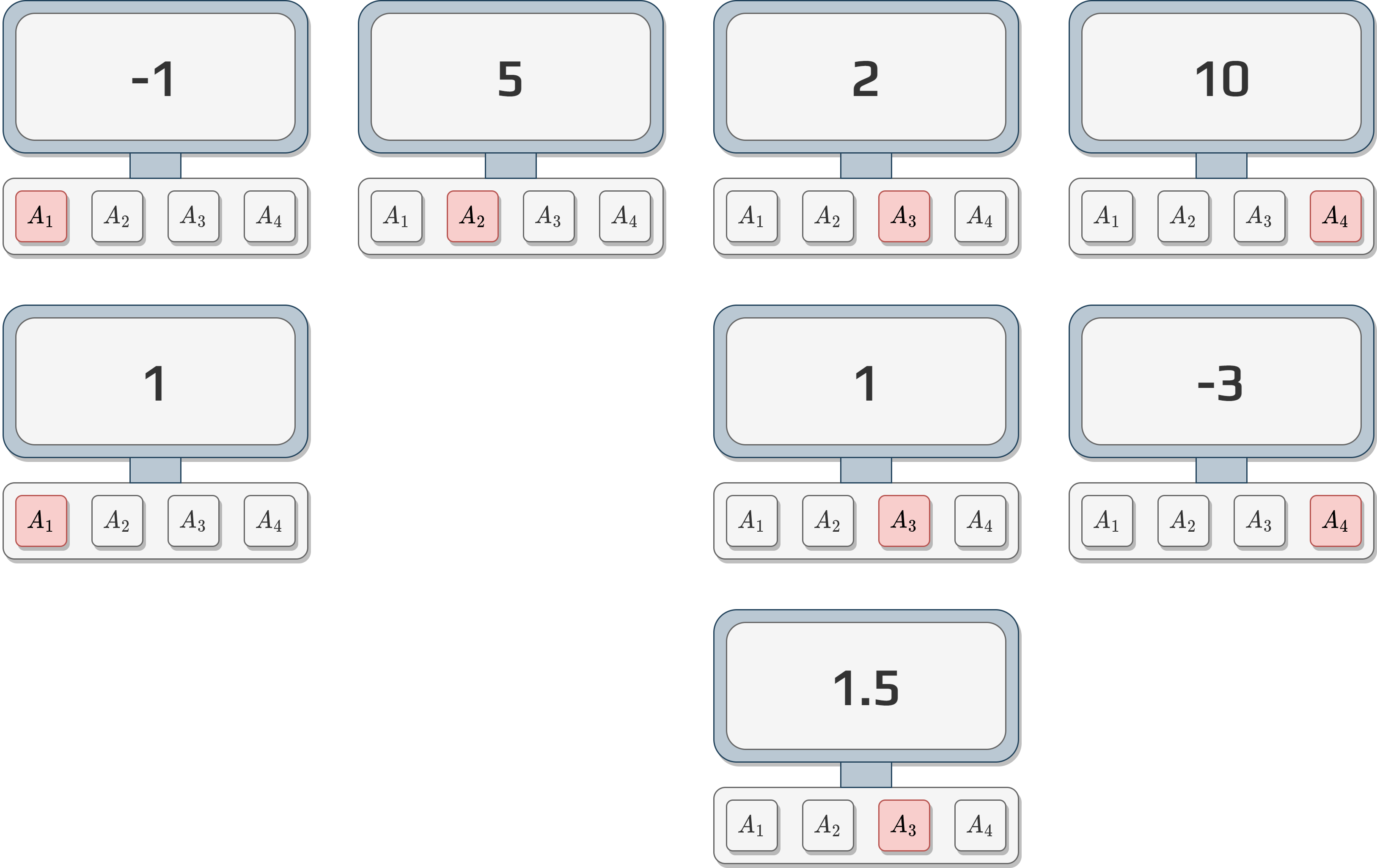
• Based on these results:

  • Decide which button (action) you would push.

  • Justify why.

• One way to estimate the expected total reward is averaging the rewards actually received:

\[Q_t(a) = \frac{\sum^{t-1}_{i=1}R_i\times \mathbb{1}_{A_t=a}}{\sum^{t-1}_{i=1}\mathbb{1}_{A_t=a}}\]

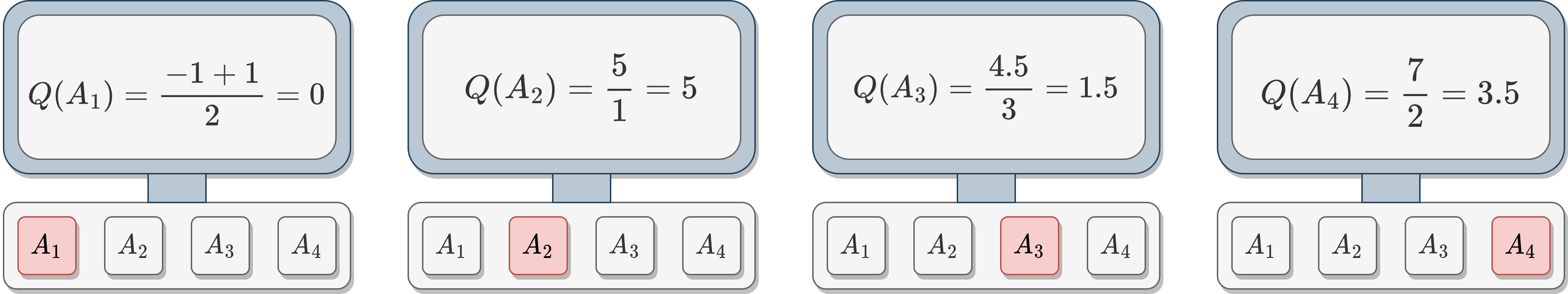
Example

If we take back the previous activity and calculate the \(Q\)-values we obtain the following.

2.2.2. Selecting the action

• Once the values are estimated, we need to have a strategy to select the action.

• Keeping in mind we want to explore and exploit.

• A good way is to mix greedy action and random actions.

  • We will select the greedy action \(1-\epsilon\) of the time.

  • Then a random action \(\epsilon\) of th time.

• It is the \(\epsilon\)-greedy method.

Important

It guarantees that it will converge, but does not give any guarantee on the performance.

Activity

• Consider the following two actions with their values:

  • \(a_1\), \(Q(a_1)=10\)

  • \(a_2\), \(Q(a_2)=1\)

• If you apply the \(\epsilon\)-greedy action selection with \(\epsilon=0.5\), what is the probability of choosing \(a_1\)?

2.3. Incremental implementation

• We need to execute each action a very large number of times.

• So, it is important to investigate how the reward can be computed efficiently.

• Consider a problem with a single action:

  • Let \(R_i\) the reward received after the \(i\text{th}\) action.

  • Let \(Q_n\) denote the estimate of this action after being selected \(n-1\) times.

• \(Q_n\) can be written:

\[Q_n = \frac{R_1 + \dots + R_{n-1}}{n-1}\]

Activity

• How would you implement that?

• What happens in terms of memory consumption and computation time?

• The most efficient way to implement that is to use an increment formula for updating the average.

• Given \(Q_n, R_n\):

\[\begin{split}\begin{aligned} Q_{n+1} &= \frac{1}{n}\sum^n_{i=1}R_i\\ &= Q_n + \frac{1}{n}\left[ R_n - Q_n \right] \end{aligned}\end{split}\]

• With this we can calculate in constant time and memory.

• This update function is a key of reinforcement learning.

• We find this form a lot:

  \[NewEstimate \leftarrow OldEstimate + StepSize\left[Target-OldEstimate\right]\]

Activity

• What represents \([Target - OldEstimate]\)?

Note

• \(StepSize\) is not the step number but the size of the step, in our case it’s \(\frac{1}{n}\).

• In reinforcement learning, it’s often \(\alpha\).

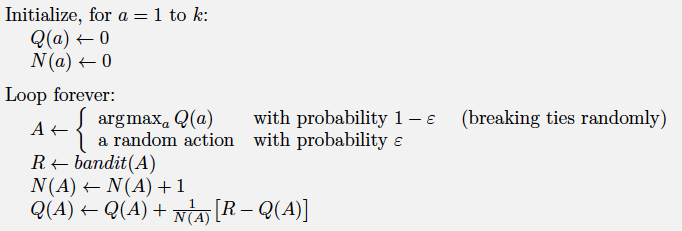
Pseudocode for the bandit problem