Applying our first RL algorithms!#
Grid World#
Let’s go back to our grid world problem, where the agent start always in the same position and needs to reach a cell in the world while avoiding the trap.
Remember that visually the world will look like this:

Now we wish to apply TD-learning to this environment and compare the results with Value Iteration.
One advantage of TD learning is that the algorithm is model-free, so we don’t need to define explicitly the transition function in the environment. No other modifications are required and we can use the environment for our experiments.
class GridWorld(gymnasium.Env):
  def __init__(self):
    # Define the action and observation spaces
    self.action_space = spaces.Discrete(4) # Up, Down, Left, Right
    self.observation_space = spaces.Discrete(12) # 12 cells
    # Initialize the state
    self.state = 0
    self.terminals = [11, 7]

  def step(self, action: int):

    self._transition(action)
    done = False
    reward = 0
    if self.state == 11:
      reward = 10
      done = True
    elif self.state == 7:
      reward = -10
      done = True
    # Return the observation, reward, done flag, and info
    return self.state, reward, done, {}

  def _transition(self, action: int):
    """
    Transition function.
    :param action: Action to take
    """
    r = np.floor(self.state / 4)
    c = self.state % 3

    prob = np.random.random()
    if prob < 0.80:
      actual_action = action
    elif prob < 0.90:
      # Adjacent cell "clockwise"
      actual_action = (action + 1) % 4
    else:
      # Adjacent cell "counter clockwise"
      actual_action = (action - 1) % 4

    if actual_action == 0:
      r = max(0, r - 1)
    elif actual_action == 2:
      r = min(2, r + 1)
    elif actual_action == 1:
      c = max(0, c - 1)
    elif actual_action == 3:
      c = min(3, c + 1)
    self.state = int(r * 4 + c)

  def reset(self):
    """
    Reset the environment.
    """
    self.state = 0
    return self.state

  def render(self, render="human"):
    fig, ax = plt.subplots()
    ax.set_xlim(0, 4)
    ax.set_ylim(0, 3)
    ax.set_aspect('equal')


    for i in range(4):
      for j in range(3):
        if j * 4 + i == 11:
          rect = Rectangle((i, j), 1, 1, edgecolor='black', facecolor='green')
          ax.add_patch(rect)
        elif j * 4 + i == 7:
          rect = Rectangle((i, j), 1, 1, edgecolor='black', facecolor='red')
          ax.add_patch(rect)
        elif j * 4 + i == 5:
          rect = Rectangle((i, j), 1, 1, edgecolor='black', facecolor='grey')
          ax.add_patch(rect)
        else:
          rect = Rectangle((i, j), 1, 1, edgecolor='black', facecolor='white')
          ax.add_patch(rect)

    ax.tick_params(axis='both',       # changes apply to both axis
                    which='both',      # both major and minor ticks are affected
                    bottom=False,      # ticks along the bottom edge are off
                    top=False,         # ticks along the top edge are off
                    left=False,
                    right=False,
                    labelbottom=False,
                    labelleft=False) # labels along the bottom edge are off

    plt.show()
SARSA#
SARSA is an online reinforcement learning algorithm, so we only need to manage one policy. The implementation is trivial, but we want to make it compatible with a Gym environment. We will only consider the \(\epsilon\)-greedy action selection, the other action-selections are left as a bonus exercise.
def greedy_action_selection(q_s, epsilon):
    rng = np.random.default_rng()
    if rng.random() > epsilon:
        return np.argmax(q_s)
    else:
        return rng.choice(len(q_s))

def sarsa(env, N: int, alpha: float, epsilon: float):
    rng = np.random.default_rng()

    # We initialize the Q-values randomly.
    # We start by generating enough random numbers for all the pair state-action.
    # Then we reshape to obtain a table with the states as rows and actions as columns.
    q = rng.normal(0, 1, env.observation_space.n * env.action_space.n).reshape((env.observation_space.n, env.action_space.n))
    # The two terminal states are sets to 0 for all the actions.
    q[env.terminals, :] = 0

    for n in range(N):
        s = env.reset()
        done = False
        a = greedy_action_selection(q[s,:], epsilon)
        while not done:
            s_next, r, done, _ = env.step(a)
            a_next = greedy_action_selection(q[s_next,:], epsilon)
            q[s, a] += alpha*(r + 0.9*q[s_next,a_next] - q[s, a])
            s = s_next
            a = a_next

    # argmax gives us the highest value for each state, so the policy.
    return np.argmax(q, axis = 1), q
import matplotlib.pyplot as plt

def plot_conv(q_s0):
    plt.style.use('seaborn-v0_8')
    x = np.linspace(0, len(q_s0), len(q_s0))

    fig, ax1= plt.subplots()
    plt.subplots_adjust(hspace=0.5)

    ax1.plot(x, q_s0, linewidth=2.0, color="C1")
    ax1.set_title("Evolution of the value of the initial state")
    ax1.set_ylabel("Value of optimal action")
    ax1.set_xlabel("Episodes")

    plt.show()
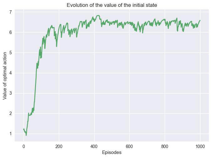
We run SARSA on our environment and save the q-values for the initial state \(s_0\). Saving the value of the initial state can help us see how fast we are converging to the optimal policy.
Note
TD-learning will theoretically converge to the optimal policy for a number of episode \(N\) sufficiently large.
Let’s see what happens!
env = GridWorld()
pi, q, q_s0 = sarsa_conv(env, 1000, 0.1, 0.5)
plot_conv(q_s0)
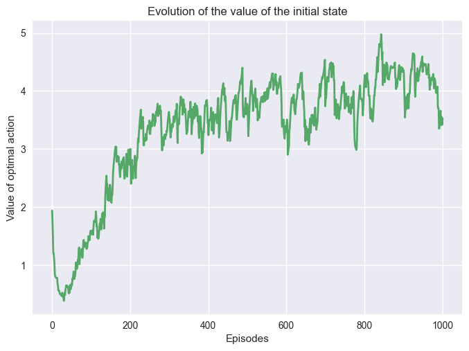
One can note that \(V(s_0)\) fluctuated a lot during the training, it is normal and expected. These fluctuations have many explanations, the first one is the action-selection method. As we explore the different actions it explores good and bad trajectories, that have an impact of the value function. Another reason comes from the model-free approach of the algorithm. The algorithm doesn’t have the transition function, so it needs to learn it during the training.
Impact of the Hyperparameters#
Most algorithm requires parameters, such as \(\epsilon\), \(\alpha\), etc. These parameters, often called hyperarameters, are essential to the learning process, and have a important impact on the quality of the learning. It is necessary to understand their purpose, and know how to tune them to obtain the desire result.
Important
The optimal value of each parameter depends of the problem. Having a combination that works for a problem doesn’t guarantee it will work for another problem. Some parameters are well studied, and are known to perform (or under perform) in specific range.
We can change the \(\epsilon\) the exploratory ratio, and it will impact the learning.
env = GridWorld()
pi, q, q_s0 = sarsa_conv(env, 1000, 0.1, 0.2)
plot_conv(q_s0)
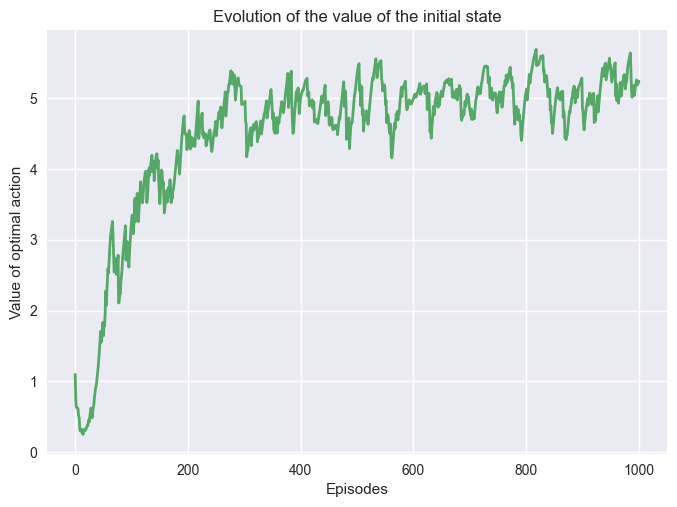
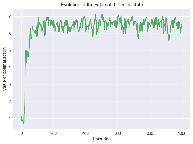
We can see that the value function converges to a higher value by the end. It doesn’t mean the policy is better! We are not evaluating the policy, we are just saving the value during training that has a bias due to the exploration. Reducing the exploration reduces the bias leading to higher values.
Now if we change the value of \(\alpha\).
env = GridWorld()
pi, q, q_s0 = sarsa_conv(env, 1000, 0.3, 0.5)
plot_conv(q_s0)
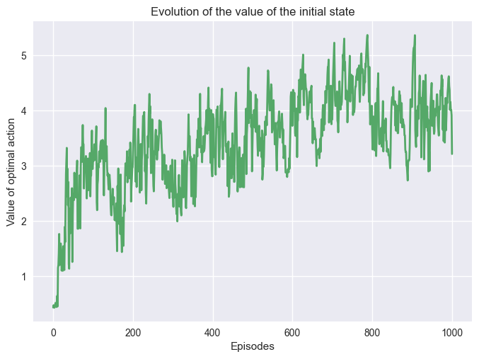
Increasing \(\alpha\) increase the size of the update. On a simple problem, it helps the convergence to the optimal policy. However, it has been proven that a step size too large can lead to a longer convergence speed.
Q-Learning#
Q-Learning is known because it is the first off-policy reinforcement learning algorithm. It works very similarly to SARSA, but as an off-policy algorithm it has two policies, the behavior policy and the target policy.
def q_learning(env, N: int, alpha: float, epsilon: float):
    rng = np.random.default_rng()

    # We initialize the Q-values randomly.
    # We start by generating enough random numbers for all the pair state-action.
    # Then we reshape to obtain a table with the states as rows and actions as columns.
    q = rng.normal(0, 1, env.observation_space.n * env.action_space.n).reshape((env.observation_space.n, env.action_space.n))
    # The two terminal states are sets to 0 for all the actions.
    q[env.terminals, :] = 0

    for _ in range(N):
        s = env.reset()
        done = False
        while not done:
            a = greedy_action_selection(q[s,:], epsilon)
            s_next, r, done, _ = env.step(a)
            q[s, a] += alpha*(r + 0.9*np.max(q[s_next, :]) - q[s, a])
            s = s_next

    # argmax gives us the highest value for each state, so the policy.
    return np.argmax(q, axis = 1), q
Let’s try the algorithm and see if there is any difference with SARSA!
env = GridWorld()
pi, q, q_s0 = q_learning_conv(env, 1000, 0.1, 0.5)
plot_conv(q_s0)
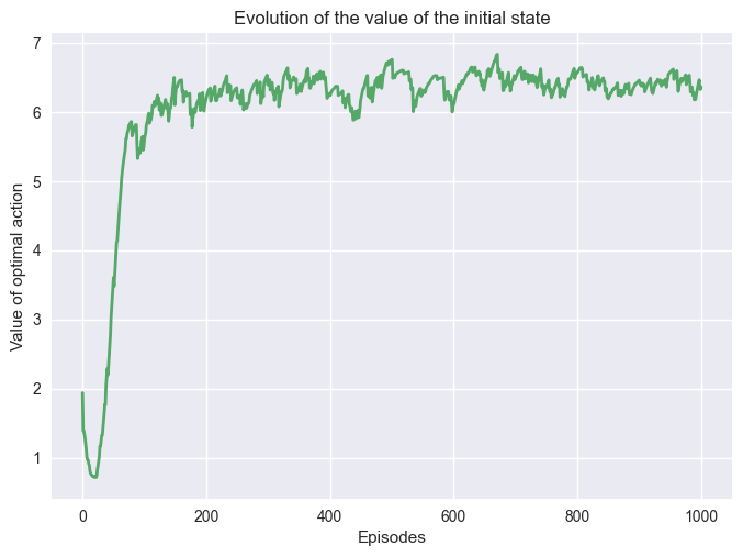
Q-Learning is surprisingly doing very well for an off-policy algorithm, and it converged very quickly compared to SARSA.
The main reason is that the problem is simple and Q-Learning is not exploring while choosing \(a'\), thus for simple problems it converges to the optimal policy very fast.
Impact of Hyperparameters#
We can also study the impact of these parameters on Q-learning, starting with \(\epsilon\).
env = GridWorld()
pi, q, q_s0 = q_learning_conv(env, 1000, 0.1, 0.2)
plot_conv(q_s0)
Reducing \(\epsilon\) reduced the exploration and led to a longer convergence period.
Let’s see how \(\alpha\) impacted the learning.
env = GridWorld()
pi, q, q_s0 = q_learning_conv(env, 1000, 0.3, 0.5)
plot_conv(q_s0)
We can see the same behavior that happened with SARSA. Increasing \(\alpha\) made the algorithm converged faster.
Analysis#
Being able to train an agent on an environment is important, but it is crucial to be able to analyze the results obtain during and after the training. RL algorithms are not always giving good results, and it is important to understand what we obtain from the training.
Training stability#
One point that is often overlooked is the stability of the training.
In the previous examples, we trained our agent and we plotted the evolution of the Q-value for \(s_0\). Obtaining a good result after one training doesn’t guarantee that if we train again with the same parameters, we will also obtain a good policy.
It two different trainings with the same parameters we could obtain very different trajectories. As the problems become larger and the algorithms more complex, the training process could be unstable. We could be lucky and obtain a good policy or unlucky and think that our methods do not work.
It is possible to verify if our training is stable by training multiple time with the same parameter and see if each training looks similar.
Example
We run 25 training of both algorithms with the following parameter:
\(N= 1000\)
\(\epsilon = 0.5\)
\(\alpha = 0.1\)
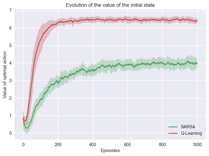
In this problem with the same parameters, we can see our training is very stable.
Evaluating the policy#
After training a policy it is necessary to evaluate the policy. Without the evaluation nothing guarantee the policy provide good results.
def evaluate(env, policy, N):
    rewards = []
    for _ in range(N):
        s = env.reset()
        done = False
        while not done:
            a = policy[s]
            s_next, r, done, _ = env.step(a)
            s = s_next
        rewards.append(r)
    return rewards
Example
We run 1000 evaluation on both algorithms after training them with the following parameter:
\(N= 1000\)
\(\epsilon = 0.5\)
\(\alpha = 0.1\)
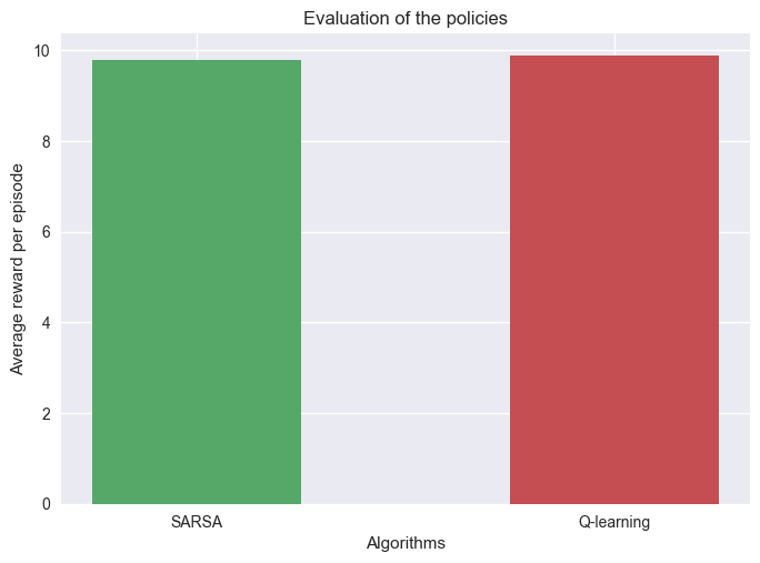
We can see that the policies perform almost gives a 100% success.
Even if the value functions of the SARSA and Q-Learning are different they still converge to an optimal policy.
Important
The value of the value functions is not enough to decide if the olicy is optimal or not. Evaluations are necessary to conclude on the performance of the policy.