Multi-armed bandit - Action Selection methods#
The algorithm updates the action-value by averaging the rewards.
This method consider that every reward has the same weights.
Another popular way in reinforcement learning is to give more weights to the more recent rewards.
Constant step-size parameter#
If we take the previous formula and we replace it with a constant parameter \(\alpha\) we obtain:
\[ Q_{n+1} = Q_n + \alpha\left[ R_n - Q_n \right] \]where the step-size parameter \(\alpha \in (0,1]\) is constant.
\(Q_{n+1}\) is called a weighted average of post rewards and initial estimate \(Q_1\):
Note
It is called a weighted average because the sum of the weights is:
Action-value initialization#
We have seen that the algorithm is initialized with some default action-value estimate \(Q_1(a)\).
This method is statistically biased by the initial estimate.
For the sampled average, the bias disappears once all actions have been selected.
However, for the weighted average, the bias is permanent. Even if it decreases over time.
Example
We can compare the sampled average and the weighted average.
We will initialize the weighted average of action 4 to something neutral like 0.
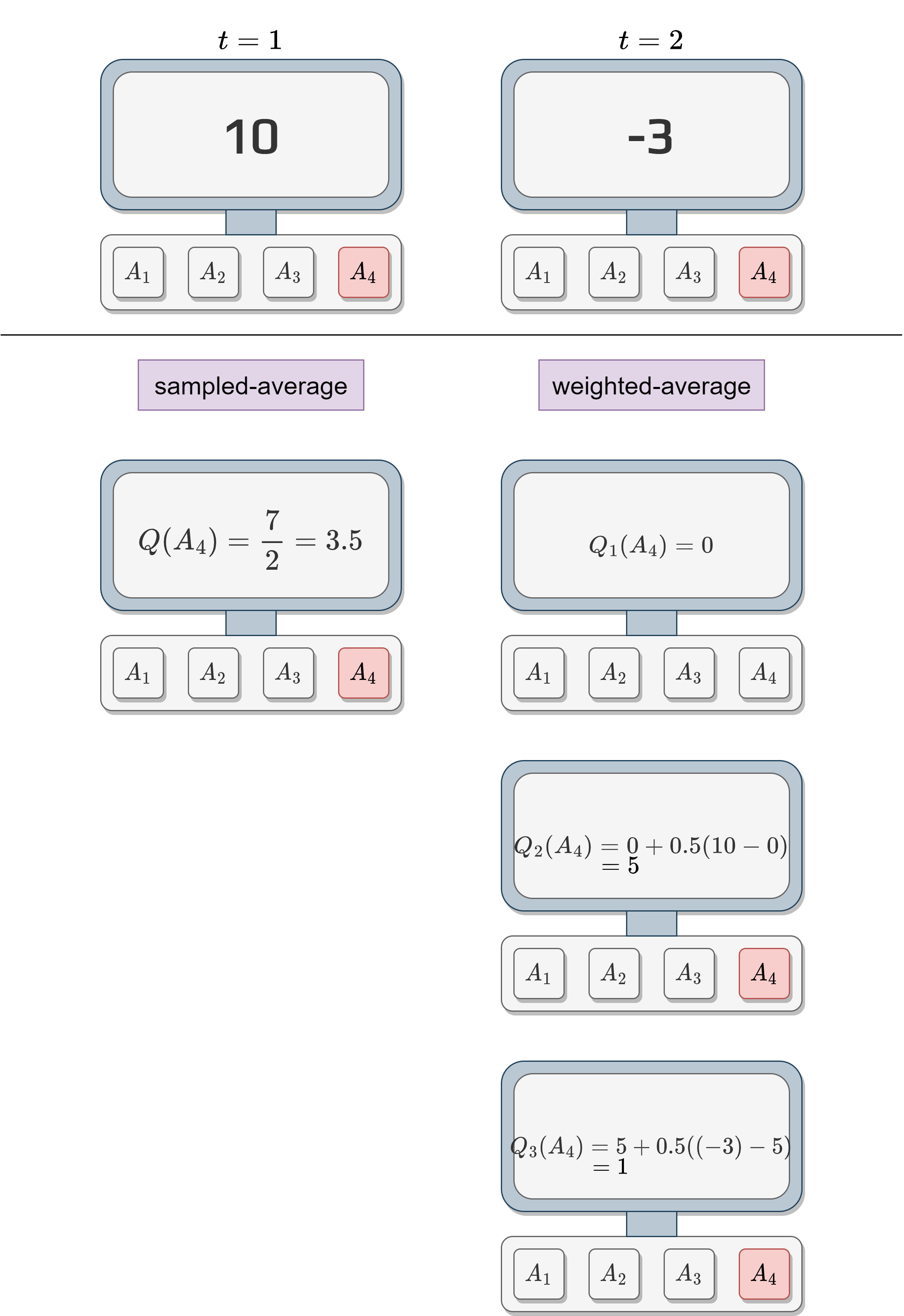
We can see that the sampled-average value and the weighted average value are not the same.
This bias cannot be overcome by choosing different initial value.
Setting all the actions to a positive value is optimistic.
After trying one action:
The algorithm will be disappointed by the returned reward (compared to the estimate).
It will select another action due to this disappointment.
Because all the actions are over optimistic, the algorithm will choose all of them multiple times.
Upper-Confidence-Bound action-selection#
Let’s think about the action-selection seen until now.
Greedy action-selection:
Always choose the action that has the higher expected reward.
It doesn’t explore.
\(\epsilon\)-greedy action-selection:
It forces the selection of non-greedy action based on a probability \(\epsilon\).
No preferences between non-greedy action.
Activity
What is the downfall of \(\epsilon\)-greedy?
It is possible to improve the action-selection by adding a few parameters to the selection algorithm.
The idea is to base the exploration on the uncertainty of the estimate.
Having a high uncertainty means that we didn’t explore the action often compared to the numbers of action selected in total.
If we don’t have a good estimate, we should explore.
We call this Upper-Confidence bound.
The action-selection formula becomes:
\[ A_t = \arg \max_a\left[ Q_t(a)+c\sqrt{\frac{\ln t}{N_t(a)}} \right] \]where
\(\ln t\) is the natural logarithm of \(t\),
\(N_t(a)\) is the number of time \(a\) has been selected,
and \(c>0\) the degree of exploration.
Activity
What happens when \(N_t(a)\) increase?
What happens when \(\ln t\) increase?
When our uncertainty on the estimate decrease the action is less selected.
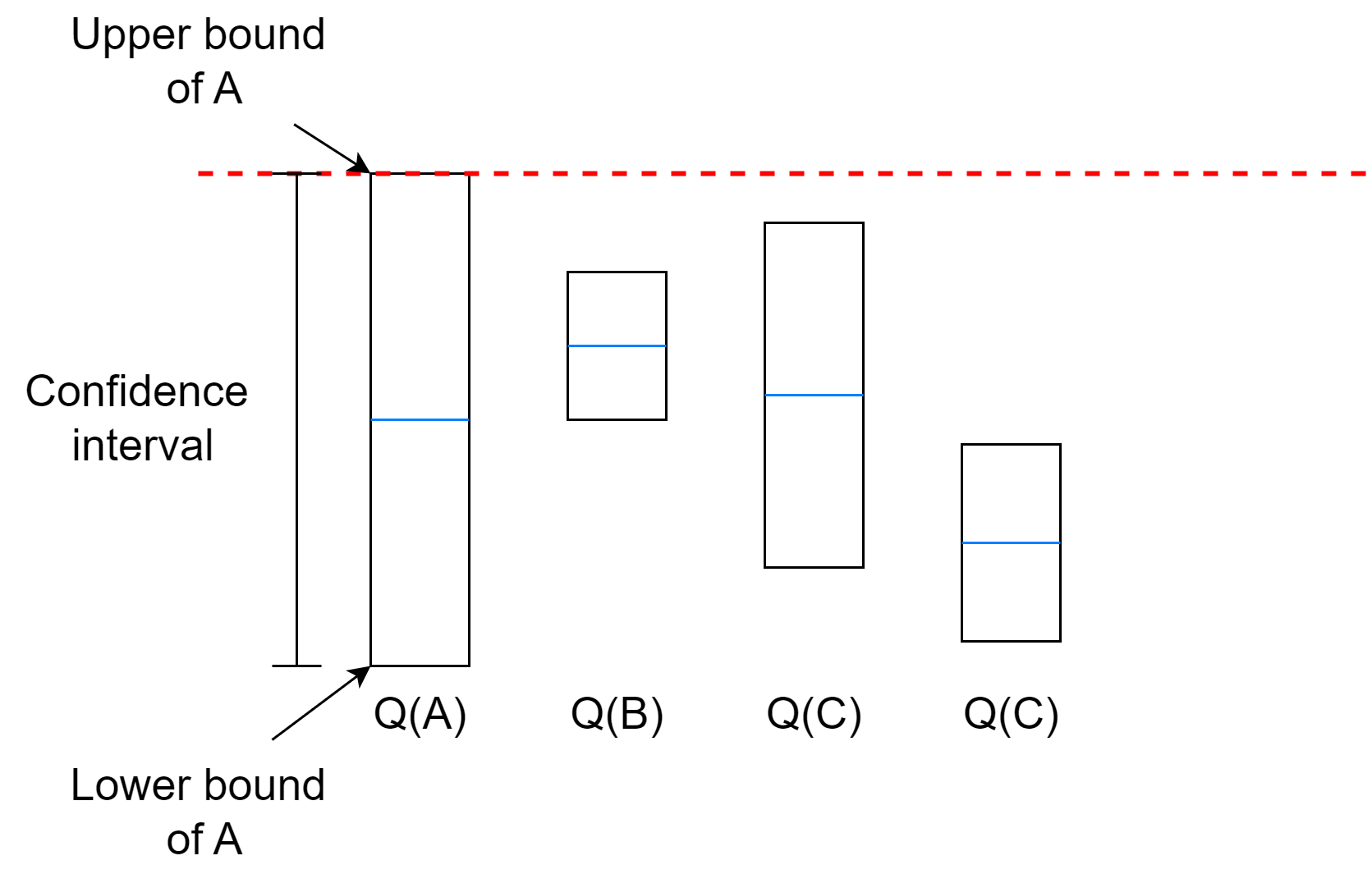
The algorithm will select the action with the highest upper bound even if the uncertainty is very high.
If multiple actions have very close upper bounds, it will depend on the exploration coefficient.
Activity
If we use our previous samples.
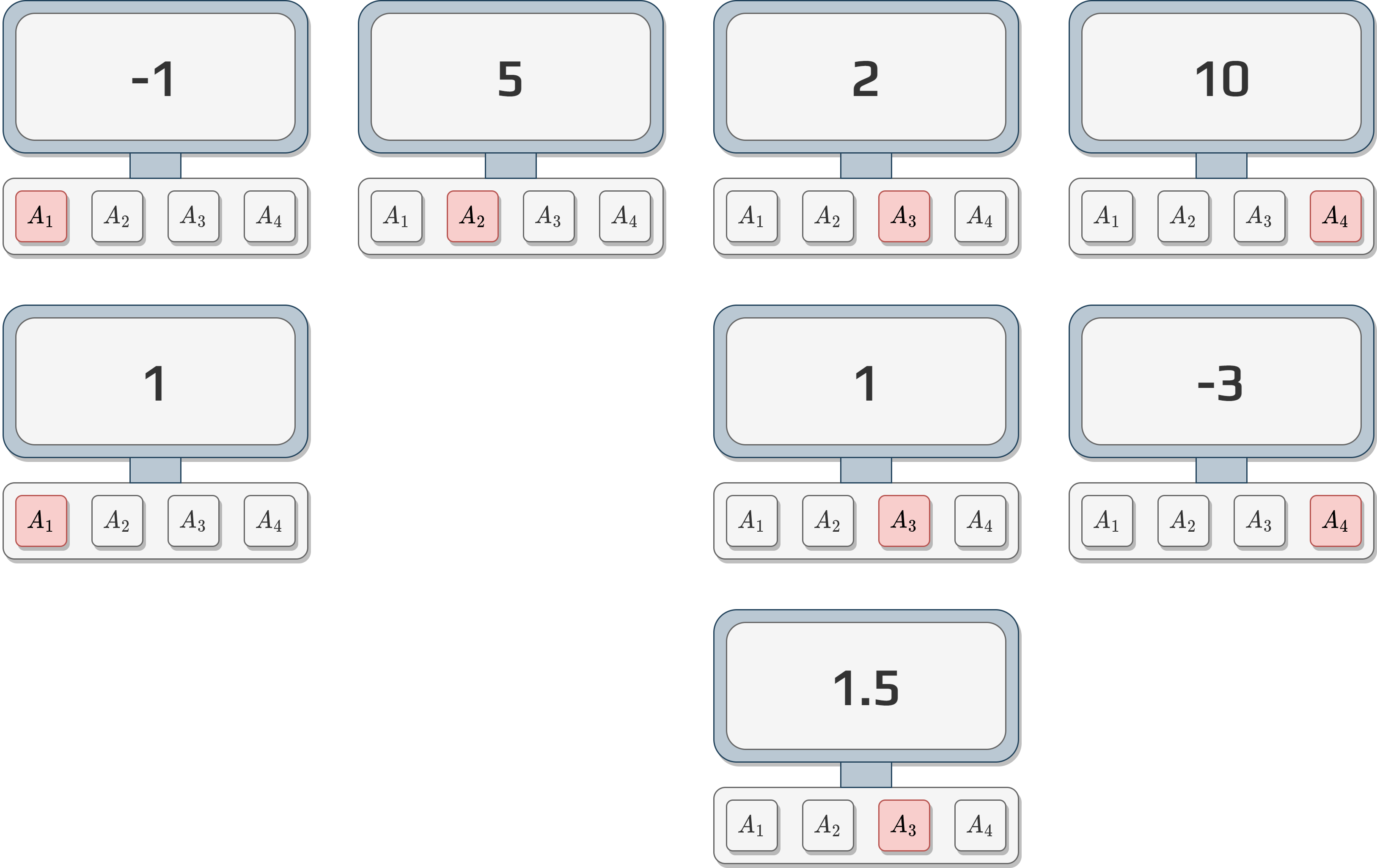
Calculate each \(Q\) values using the weighted average.
Use UCB with \(c=2\) to decide what will be the next action.
Theoretical Guarantees of UCB#
UCB is not just a heuristic - it has strong theoretical foundations
It provides regret bounds: guarantees on how much worse it performs compared to always choosing the optimal action
Regret Definition:
Let \(r^* = \max_a q_*(a)\) be the value of the optimal action
The regret at time \(T\) is: \(R_T = \sum_{t=1}^T (r^* - q_*(A_t))\)
This measures the total “loss” from not always choosing the best action
UCB Regret Bound:
UCB achieves regret of \(O(\sqrt{k \ln T})\) where \(k\) is the number of actions
This is logarithmic in time - very good performance!
The regret grows slowly even for long runs
Why This Matters
This bound tells us that UCB will eventually find the optimal action and the cost of exploration decreases over time. No algorithm can do fundamentally better than this bound.
Gradient Bandit Algorithms#
All previous methods have one thing in common.
They all based the action-selection on received rewards.
We will discuss another technic based on the preference of an action \(a\), \(H_t(a)\).
Higher the preference is, more often the action is selected.
We use this preference in a softmax distribution:
\[ P(A_t=a)=\frac{e^{H_t(a)}}{\sum_{b=1}^{k}e^{H_t(b)}}=\pi_t(a) \]where \(\pi_t(a)\) is the probability to select \(a\) at time \(t\).
Now, we need to calculate the preference \(H_t(a)\).
At the beginning \(H_1(a) =0, \forall a \in A\).
We use stochastic gradient ascent.
After each action \(A_t\) the preference is updated:
\[\begin{split} \begin{aligned} H_{t+1}(A_t) &= H_t(A_t) + \alpha(R_t - \bar{R}_t)(1-\pi_t(A_t))\text{, and}\\ H_{t+1}(a) &= H_t(a) - \alpha(R_t - \bar{R}_t)\pi_t(a)\text{, for all } a \neq A_t \end{aligned} \end{split}\]where \(\alpha >0\) is the step-size parameter, \(\bar{R}_t \in \mathbb{R}\) is the average reward not including time \(t\).
We often refer to \(\bar{R}_t\) as the baseline.
Activity
What happens if the reward is greater than the baseline?
What happens if the reward is less than the baseline?
Thompson Sampling#
Thompson Sampling takes a completely different approach to the exploration-exploitation problem.
Instead of using confidence intervals or preferences, it uses Bayesian inference.
The key idea: maintain a probability distribution over the true value of each action.
The Bayesian Approach#
For each action \(a\), we maintain a belief about its true value \(q_*(a)\).
This belief is represented as a probability distribution.
When we need to choose an action, we sample from these distributions and pick the action with the highest sample.
Algorithm Details#
We assume each action’s reward follows a normal distribution with unknown mean \(\mu_a\) and known variance \(\sigma^2\).
Our belief about \(\mu_a\) is also a normal distribution: \(\mu_a \sim \mathcal{N}(\hat{\mu}_a, \hat{\sigma}_a^2)\).
At each time step:
Sample a value \(\theta_a\) from each action’s belief distribution
Select the action with the highest sampled value: \(A_t = \arg\max_a \theta_a\)
Update the belief distribution for the selected action using Bayesian inference
Bayesian Update#
After receiving reward \(R_t\) for action \(A_t\), we update our belief:
The posterior mean becomes: $\( \hat{\mu}_{A_t} \leftarrow \frac{\hat{\sigma}_{A_t}^2 R_t + \sigma^2 \hat{\mu}_{A_t}}{\hat{\sigma}_{A_t}^2 + \sigma^2} \)$
The posterior variance becomes: $\( \hat{\sigma}_{A_t}^2 \leftarrow \frac{\hat{\sigma}_{A_t}^2 \sigma^2}{\hat{\sigma}_{A_t}^2 + \sigma^2} \)$
Why Thompson Sampling Works#
Natural exploration: Actions with higher uncertainty get sampled more often
Probability matching: The probability of selecting an action equals the probability it’s optimal
No tuning parameters: Unlike \(\epsilon\)-greedy or UCB, no exploration parameter to tune
Activity
Compare Thompson Sampling to UCB: both use uncertainty to drive exploration. What’s the key difference in how they use this uncertainty?
What happens to the belief distributions as we collect more data?
Algorithm Comparison#
Now that we’ve covered the main bandit algorithms, let’s compare them:
Algorithm |
Exploration Strategy |
Parameters |
Computational Cost |
Best Use Case |
|---|---|---|---|---|
ε-greedy |
Random exploration with probability ε |
ε (exploration rate) |
Very Low |
Simple baseline, when you want interpretable behavior |
UCB |
Confidence-based exploration |
c (exploration coefficient) |
Low |
When you want principled exploration without tuning |
Gradient Bandit |
Preference-based softmax |
α (step size), baseline |
Medium |
When action values vary significantly |
Thompson Sampling |
Bayesian probability matching |
None (prior parameters) |
Medium |
When you want optimal exploration and can handle Bayesian updates |
When to Use Which Algorithm?#
Use ε-greedy when:
You need a simple, interpretable baseline
Computational resources are extremely limited
You have a good intuition for setting ε
Use UCB when:
You want theoretically grounded exploration
You don’t want to tune parameters extensively
The problem has stationary rewards
Use Gradient Bandit when:
Action values have very different scales
You want to learn relative preferences
The environment is non-stationary
Use Thompson Sampling when:
You want near-optimal exploration
You can handle the computational overhead
You have prior knowledge about reward distributions
Activity
Consider these scenarios and choose the best algorithm:
A clinical trial where you want to minimize patient harm while finding the best treatment
An A/B test for website optimization with limited computational budget
A recommendation system where user preferences change over time
Theoretical Foundations and Performance Guarantees#
Understanding the theoretical properties of bandit algorithms helps us choose the right one and understand their limitations.
Regret Analysis#
What is regret?
Regret measures how much worse an algorithm performs compared to an oracle that always picks the optimal action
Formally: \(\text{Regret}_T = T \cdot r^* - \sum_{t=1}^T R_t\)
Where \(r^* = \max_a q_*(a)\) is the optimal expected reward
Why regret matters:
Lower regret = better performance
Regret bounds tell us worst-case guarantees
Help compare algorithms theoretically
Algorithm Performance Guarantees#
Algorithm |
Regret Bound |
Key Property |
|---|---|---|
Random |
\(O(T)\) |
Linear regret - very bad |
ε-greedy |
\(O(T)\) |
Can get stuck in suboptimal actions |
UCB |
\(O(\sqrt{k \ln T})\) |
Logarithmic dependence on time |
Thompson Sampling |
\(O(\sqrt{kT})\) |
Optimal for many distributions |
Interpreting the bounds:
\(O(\sqrt{k \ln T})\) grows much slower than \(O(T)\)
UCB’s logarithmic factor makes it very efficient for long runs
Thompson Sampling is optimal for Bernoulli rewards
Lower Bounds - Fundamental Limits#
No algorithm can do better than:
\(\Omega(\sqrt{kT})\) regret in the worst case
This means there are fundamental limits to how well any algorithm can perform
UCB and Thompson Sampling achieve near-optimal performance
Key Insight
The exploration-exploitation trade-off has mathematical limits. No algorithm can eliminate the cost of exploration entirely - you must pay some price to learn about the environment.
Practical Implications#
For practitioners:
UCB provides strong guarantees with simple implementation
ε-greedy has poor theoretical guarantees but works well in practice with good ε
Thompson Sampling is theoretically optimal for specific cases
Random exploration should be avoided - it’s provably bad
Parameter selection guidance:
UCB: \(c = \sqrt{2}\) is theoretically motivated
ε-greedy: ε should decrease over time (e.g., \(\epsilon_t = 1/t\)) for better regret
Thompson Sampling: Prior choice affects finite-time performance but not asymptotic regret
From Bandits to Full Reinforcement Learning#
Having mastered multi-armed bandits, you’re now ready to understand how they connect to the broader reinforcement learning framework.
What Bandits Taught Us#
Through bandits, we’ve learned fundamental concepts that apply to all RL:
Core Concepts Mastered:
Exploration vs Exploitation: The need to balance trying new actions with using known good ones
Value Estimation: How to estimate the worth of actions from limited experience
Action Selection: Different strategies for choosing actions based on current knowledge
Learning from Experience: How to update beliefs based on observed rewards
Limitations of Bandits#
Bandits are powerful but limited:
Single State: All decisions happen in the same context
Immediate Rewards: Feedback is instant - no delayed consequences
Independent Actions: Each action choice doesn’t affect future situations
Stationary Environment: The world doesn’t change based on your actions
The Jump to Full RL#
Full reinforcement learning removes these limitations:
Multiple States:
The agent can be in different situations (states)
Each state may have different optimal actions
The agent must learn a policy: what to do in each state
Sequential Decision Making:
Actions in one state lead to new states
Current decisions affect future options
Must consider long-term consequences, not just immediate rewards
Delayed Rewards:
Actions may have consequences many steps later
Must solve the credit assignment problem: which past actions deserve credit for current rewards?
Connecting the Concepts#
Key Insight
Every state in a full RL problem can be thought of as a separate bandit problem!
The challenge is that:
You have many bandits (one per state)
The bandits are connected (actions in one affect others)
Rewards may come much later
Mathematical Connection:
Bandit: \(Q(a)\) - value of action \(a\)
Full RL: \(Q(s,a)\) - value of action \(a\) in state \(s\)
Preview: What’s Coming Next#
In the next section, we’ll explore Markov Decision Processes (MDPs), which provide the mathematical framework for full RL:
States: All possible situations the agent can encounter
Actions: Available choices in each state
Transitions: How actions move you between states
Rewards: Feedback that may be delayed
Policies: Complete strategies for all states
The exploration-exploitation trade-off you’ve mastered in bandits becomes even more complex when decisions have long-term consequences!
Activity
Before moving on, think about these questions:
How would you modify ε-greedy if you had 1000 different states instead of just 1?
If rewards come 10 steps after actions, how would this change your learning approach?
What new challenges arise when your actions change which states you can visit?