Introduction to Neural Networks#
Neural Networks (NN) are a foundational tool in machine learning, including reinforcement learning. To effectively understand and apply NNs, we begin with an introduction to the necessary mathematical background: Linear Algebra.
Linear Algebra#
Linear algebra is deeply linked with neural networks. A solid understanding of its concepts is essential for creating and working with NNs.
Scalars, Vectors, Matrices, and Tensors#
The study of linear algebra involves several types of mathematical objects.
Scalars
Definition 13 (Scalar)
A scalar is a single number defined on a domain.
Notation: Scalars are denoted by italic lowercase letters, e.g., \(s \in \mathbb{R}\).
Vectors
Definition 14 (Vector)
A vector is an ordered array of numbers, where each number is identified by its position in the sequence.
Notation: Vectors are denoted by bold lowercase letters, e.g., \(\mathbf{x}\).
Elements: Each element is represented by the vector name subscripted with its index, e.g., \(x_1, x_2, \ldots\).
When written explicitly, vectors appear as columns enclosed in square brackets:
\[\begin{split}\mathbf{x} = \begin{bmatrix} x_1 \\ x_2 \\ \vdots \\ x_n \end{bmatrix}\end{split}\]
Matrices
Definition 15 (Matrix)
A matrix is a two-dimensional array of numbers, where each element is identified by two indices.
Notation: Matrices are denoted by bold uppercase letters, e.g., \(\mathbf{A}\).
Elements: Matrix elements are represented by their name in italics with indices, e.g., \(A_{m,n}\).
When written explicitly, matrices are shown as arrays enclosed in square brackets:
\[\begin{split}\mathbf{A} = \begin{bmatrix} A_{1,1} & A_{1,2} \\ A_{2,1} & A_{2,2} \end{bmatrix}\end{split}\]
Tensors
Definition 16 (Tensor)
A tensor is an \(n\)-dimensional array of numbers, where each element is identified by \(n\) indices.
Notation: Tensors are generalized multi-dimensional arrays, often denoted with boldface names.
Elements: Tensor elements are represented by their name in italics with indices, e.g., \(A_{i,j,k}\).
Operations#
With these mathematical objects, we can do different operations.
Basic Operations#
One important operation on matrices is the transpose.
The transpose of a matrix is the mirror image across the main diagonal. We denote the transpose of matrix \(\mathbf{A}\), as \(\mathbf{A}^\intercal\), such that \(\left(\mathbf{A}^\intercal\right)_{i,j} = A_{j,i}\).
Example 7 (Transpose example)
It can be verified with a small python code.
import numpy as np

A = np.array([[1, 2],
              [3, 4],
              [5, 6]])
print(np.transpose(A))
[[1 3 5]
 [2 4 6]]
We can also add matrices to each other, as long as they have the same shape. Consider two matrices \(\mathbf{A} \in \mathbb{R}^{m\times n}\) and \(\mathbf{B} \in \mathbb{R}^{m\times n}\), then \(\mathbf{C} = \mathbf{A} + \mathbf{B}\), where \(C_{i,j} = A_{i,j} + B_{i,j}\).
import numpy as np

A = np.array([[1, 2],
              [3, 4],
              [5, 6]])

B = np.array([[10, 11],
              [12, 13],
              [14, 15]])
print(A+B)
[[11 13]
 [15 17]
 [19 21]]
We can also add or multiply a scalar to matrix, such as \(\mathbf{D} = a \cdot \mathbf{B} + c\), where \(D_{i,j} = a \cdot B_{i,j} + c\).
Similarly, we can verify ot by running some python code.
import numpy as np

A = np.array([[1, 2],
              [3, 4],
              [5, 6]])

print(2*A-1)
[[ 1  3]
 [ 5  7]
 [ 9 11]]
Multiplying Matrices and Vectors#
The matrix product of matrices \(\mathbf{A}\) and \(\mathbf{B}\) is a third matrix \(\mathbf{C}\). To be defined, \(\mathbf{A}\) must have the same number of columns as \(\mathbf{B}\) has rows. Concretely if \(\mathbf{A}\in \mathbb{R}^{m\times n}\), and \(\mathbf{B}\in \mathbb{R}^{n\times p}\), then \(\mathbf{C}\in \mathbb{R}^{m\times p}\).
We can perform matrix multiplication by placing two matrices together, for example: \(\mathbf{C} = \mathbf{A}\mathbf{B}\).
The product operation is defined by:
In the following code we have \(A\in \mathbb{R}^{3\times 2}\), and \(B\in \mathbb{R}^{2\times 4}\), so the result matrix will be \(C\in \mathbb{R}^{3\times 4}\).
import numpy as np

A = np.array([[1, 2],
              [3, 4],
              [5, 6]])

B = np.array([[2, 3, 1, 4], [2, 2, 1, 5]])

print(np.matmul(A,B))
[[ 6  7  3 14]
 [14 17  7 32]
 [22 27 11 50]]
Not to mistake it with the element-wise product denoted \(\mathbf{A}\odot \mathbf{B}\).
import numpy as np

A = np.array([[1, 2],
              [3, 4],
              [5, 6]])

B = np.array([[2, 3],
              [1, 2],
              [2, 1]])

print(A*B)
[[ 2  6]
 [ 3  8]
 [10  6]]
It is now enough information to write a system of linear equations:
where \(\mathbf{A}\in \mathbb{R}^{m\times n}\) is known matrix, \(\mathbf{b}\in \mathbb{R}^{m}\) is known vector, and \(\mathbf{x}\in \mathbb{R}^{n}\) is a vector of unknown variables.
Each element \(x_i\) of \(\mathbf{x}\) is an unknown variable, and each row of \(\mathbf{A}\) and each element of $\mathbf{b} provide another constraint.
We can rewrite the previous equation as:
or even more explicitly:
Note
Matrix-vector product notation provides a more compact representation for equations of this form.
Solving Linear Equations#
We have seen linear algebra can be used to represent a system of equations, but it can also be used to solve them.
Definition 17 (Identity Matrix)
An identity matrix \(\mathbf{I}\) is a matrix that doesn’t change any vector, when multiplying the vector by that matrix. Formally, \(\mathbf{I} \in \mathbf{R}^{n\times n}\) and,
Example 8 (Idendity matrix for \(n=3\))
For example \(\mathbf{I_3}\) is \(\begin{bmatrix} 1 & 0 & 0\\ 0 & 1 & 0\\ 0 & 0 & 1\end{bmatrix}\).
Using the identity matrix we can define another tool called matrix inversion.
Definition 18 (Matrix Inverse)
The matrix inverse of \(\mathbf{A}\) is denoted \(\mathbf{A}^{-1}\), and defned such as:
It is now possible to solve our system of equations following these steps:
import numpy as np
from numpy.linalg import inv

A = np.array([[1, 1, 1],
              [0, 2, 5],
              [2, 5, -1]])

b = np.array([6, -4, 27])
ainv = inv(A)

x = np.matmul(ainv, b)
print(x)
[ 5. 3. -2.]
Important
For \(\mathbf{A}^{-1}\) to exist, the equation must have exactly one solution for every value of \(\mathbf{b}\).
Deep Neural Networks#
In previous topic, we saw that we could calculate an approximate value function \(\hat{v}(s,\mathbf{w})\). The weight vector \(\mathbf{w}\) is learned by using a gradient descent method.
This approach represents \(\hat{v}(s,\mathbf{w})\) by a linear function with respect to the feature vector \(\mathbf{x}(s)\), and finding a states features can be non-trivial.
In contrast to linear function approximation, deep learning provides a universal method for function approximation that is able to automatically learn feature representations of states, and is able to represent non-linear, complex functions that can generalize to novel states.
Feedforward Neural Networks#
Feed forward networks (FFN) are the most common type of networks in RL. FFN are built in layers with the first layer processing the input \(\mathbf{x}\) and any subsequent layer processing the output of the previous layer.
Each layer is defined as a parameterized function, and is composed of many units. The output is the concatenation of each unit output.
Usually we refer to some layers with specific terms:
Input layer: first layer of the network.
Output layer: Last layer of the network.
Hidden layers: All layers between the input and output layers.
Example 9 (FFN example)
Consider a neural network with three layers:
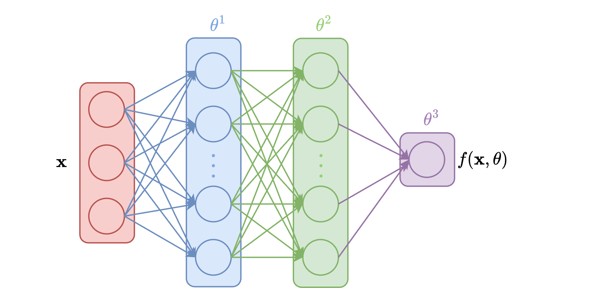
This FFN could be written as:
where \(\theta^k\) are the parameters of layer \(k\) and \(\theta = \bigcup_k \theta^k\).
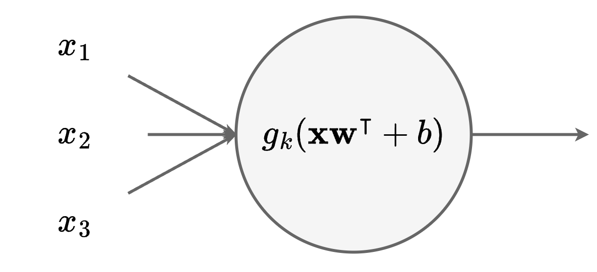
Neural Unit#
A neural unit of a layer \(k\) represents a parameterized function \(f_{k,u}: \mathbb{R}^{d_{k-1}} \rightarrow \mathbb{R}\), where \(d_{k}\) is the number of units at the layer depth \(k\).
Each unit computes a linear transformation followed by a non-linear activation function \(g_k\).
The linear transformation is computed following:
where \(\mathbf{w} \in \mathbb{R}^{d_{k-1}}\) is a weight vector, and \(b\in \mathbb{R}\) is a bias.
Important
The parameters \(\theta^k_u\in \mathbb{R}^{d_{k-1}+1}\) contains the weight vector \(\mathbf{w}\) and the bias \(b\).
So the unit computation can be written as:
Important
Activation function are crucial.
The composition of linear functions only result in a linear function.
Adding a non-linear activation function between layers allow the network to learn complex non-linear aproximations.
Example 10 (Neural Unit example)
Consider a neural unit receiving a vector \(\mathbf{x} \in \mathbb{R}^3\).
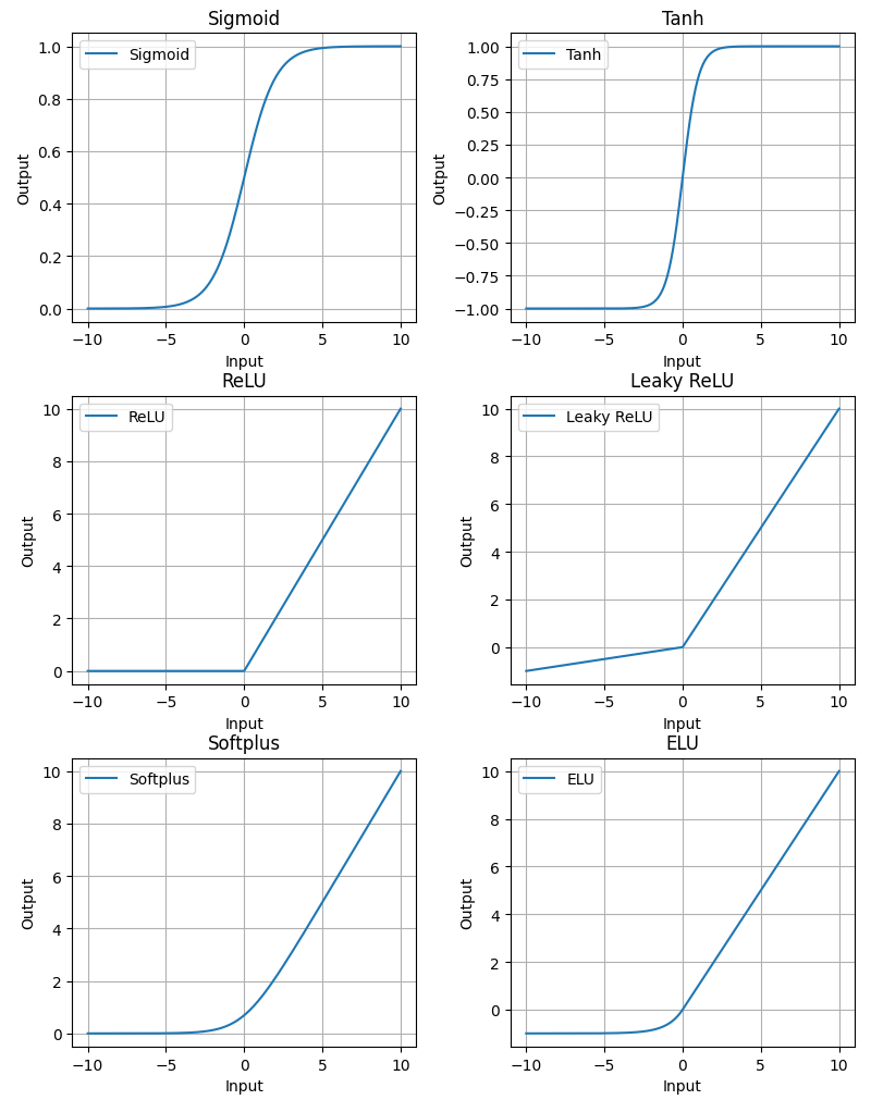
Activation Functions#
There are many activation functions, some are more common than others.
In RL, ReLU or rectified linear unit applies a non-linear transformation but remains “close to linear”. This has useful implications for gradient-based optimization. Also ReLU is able to output zero values.
The tanh and sigmoid activation functions are mostly used to restrict the output of a neural network to be within the ranges of \((-1,1)\) or \((0,1)\), respectively.
Network Composition#
A neural network is composed of several layers, and each layer is composed of neural units (neurons).
The \(k\)-th layer of a FFN receives the output of the previous layer \(\mathbf{x}_{k-1}\in \mathbb{R}^{d_{k-1}}\) and computes an output \(\mathbf{x}_k \in \mathbb{R}^{d_k}\).
If we aggregate all the neural units of the \(k\)-th layer we can write its computation as:
where \(g_k\) is the activation function, \(\mathbf{W}\in \mathbb{R}^{d_{k-1}\times d_k}\) the weight matrix, and \(\mathbf{b}_k\in \mathbb{R}^{d_k}\) the bias vector.
Note
The parameters \(\theta_k\) contains the weight matrix and the bias vector, such as \(\theta^k = \mathbf{W}\cup \mathbf{b}_k\).
This can be seen as the parallel computation of the \(d_k\) neural units.
Let’s practice#
Consider an iput \(\mathbf{x}_0 = \begin{bmatrix} 1 \\ 2 \\ 3 \end{bmatrix}\), a weight matrix \(\mathbf{W} = \begin{bmatrix} 1 & -1 & 0 \\ 2 & 0 & 1 \\ 1 & -0.3 & -1 \end{bmatrix}\), and a bias vector \(\mathbf{b} = \begin{bmatrix} -0.2 \\ 0.2 \\ 0 \end{bmatrix}\).
Let’s consider the code to calculate the output \(x_{1,1}\) of one neural unit:
x = np.array([1, 2, 3])

w_1 = np.array([1, -1, 0])
b_1 = -0.2

x1_1 = np.matmul(x,w_1.T) + b_1

print("x1_1: ", x1_1)
x1_1: -1.2
Now we can add the remaining two units:
x = np.array([1, 2, 3])

w_2 = np.array([2, 0, 1])
b_2 = 0.2

x1_2 = np.matmul(x,w_2.T) + b_2

print("x1_2: ", x1_2)


x = np.array([1, 2, 3])

w_3 = np.array([1, -0.3, -1])
b_3 = 0

x1_3 = np.matmul(x,w_3.T) + b_3

print("x1_3: ", x1_3)
x1_2:  5.2
x1_3:  -2.6
Now let’s try to calculate for the full layer containing the three neural units:
x = np.array([1, 2, 3])

W = np.array([[1, -1, 0],
              [2, 0, 1],
              [1, -0.3, -1]])

b = np.array([-0.2, 0.2, 0])

x1 = np.matmul(x,W.T) + b
print("x1: ", x1)
x1: [-1.2 5.2 -2.6]
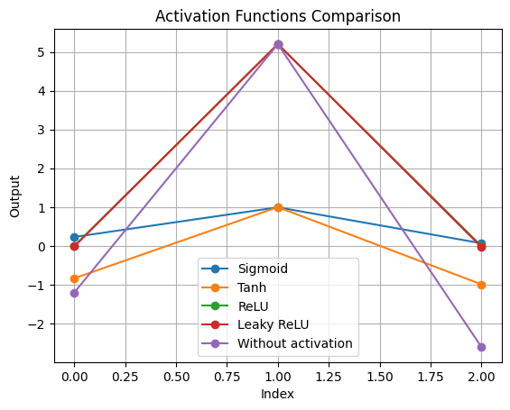
It is now possible to apply different activation functions. We will consider the sigmid, the tanh, Relu, and Leaky ReLu.
import numpy as np
import matplotlib.pyplot as plt


# Activation functions
def sigmoid(x):
    return 1 / (1 + np.exp(-x))

def tanh(x):
    return np.tanh(x)

def relu(x):
    return np.maximum(0, x)

def leaky_relu(x, alpha=0.01):
    return np.where(x > 0, x, x * alpha)

# Apply activation functions
x1_sigmoid = sigmoid(x1)
x1_tanh = tanh(x1)
x1_relu = relu(x1)
x1_leaky_relu = leaky_relu(x1)

# Plot each activation function result
activation_functions = {
    "Sigmoid": x1_sigmoid,
    "Tanh": x1_tanh,
    "ReLU": x1_relu,
    "Leaky ReLU": x1_leaky_relu,
    "Without activation": x1
}

# Plot all activation functions on the same plot
plt.figure()

for name, result in activation_functions.items():
    plt.plot(result, marker='o', label=name)

plt.title('Activation Functions Comparison')
plt.xlabel('Index')
plt.ylabel('Output')
plt.legend()
plt.grid()
Training Neural Networks#
Training neural networks involves optimizing their parameters to minimize a loss function. This process typically uses gradient-based optimization methods.
The principle is identical to the previous methods covered.
Definition 19 (Loss Function)
A loss function \(\mathcal{L}(\theta)\) measures how well the network performs on the training data with parameters \(\theta\).
We have seen the main one for value functions: Mean Squared Error (MSE).
To update the parameters \(\theta\), we also use the gradient descent algorithm.
Algorithm 17 (Gradient Descent)
Initialize parameters \(\theta\)
Repeat until convergence:
Compute gradient: \(\nabla_\theta L(\theta)\)
Update parameters: \(\theta \leftarrow \theta - \alpha \nabla_\theta L(\theta)\)
where \(\alpha\) is the learning rate.
Mini-batch Training#
In practice, computing the gradient over the entire trajectories is computationally expensive. Mini-batch training addresses this by:
Dividing the dataset into small batches
Computing gradients on each batch
Updating parameters more frequently
Algorithm 18 (Mini-batch Gradient Descent)
Initialize parameters \(\theta\)
For each epoch:
Shuffle training data
Split data into mini-batches
For each mini-batch \(B\):
Compute gradient: \(\nabla_\theta \mathcal{L}_B(\theta)\)
Update parameters: \(\theta \leftarrow \theta - \alpha \nabla_\theta \mathcal{L}_B(\theta)\)
Advantages of Mini-batch Training:
More frequent parameter updates
Better convergence behavior
More efficient use of computational resources
Backpropagation#
Backpropagation is an efficient algorithm for computing gradients in neural networks. It applies the chain rule of calculus to propagate gradients backward through the network.
Definition 20 (Backpropagation)
An algorithm that efficiently computes the gradient of the loss with respect to each parameter by working backward from the output layer to the input layer.
Once we calculate the loss, we propagate gradients backward through each layer, then we update parameters using computed gradients.