Let’s practice#
Gym environment#
It is time to practice what we have seen so far. We explained before, that the agent interacts with an environment. In this chapter, the environment is the multi-armed bandit problem. If we want to train an agent, we will need to implement the environment.
In our case we will implement the environment using the library Gymnasium (or Gym).
We will start by importing the library we need.
import numpy as np
import gymnasium as gym
from gymnasium.spaces import Discrete
Gym environment.#
Gym environments have many built-in methods we can override, but for now we will only need a few.
Every
gymenvironment must inherit from the classEnv.__init__initialize the environment: the constructor.The method
stepexecute the action sent by the agent.
All your environment will looks like this:
class MyEnv(gym.Env):

    def __init__(self):
        pass
        #  Initialize the variables you need.

    def step(self, action):
        pass
        #  Execute an action.
Then we create the environment as any other object.
my_env = MyEnv()
Multi-armed Bandit#
Now we can implement the multi-armed bandit. The code is very simple, but it will illustrate how environment are implemented.
Constructor#
In the constructor we will define:
the number of actions
how they will behave
In the bandit problem, each action have a hidden value. We could define them manually or in this example we can generate them randomly.
Let’s see the code:
def __init__(self, nb_actions):
    self.action_space = Discrete(nb_actions)
    self.q_a = np.random.default_rng().normal(0, 1, nb_actions)
You can notice a few things:
Discreteis a “type” in thegymlibrary that defines a variable that can take discrete values. In this case between 0 andnb_actions.np.random.default_rng().normal(0, 1, nb_actions)generates a list ofnb_actionsvalues between 0 and 1.
Note
We name the list q_a because we are generating the expected rewards \(q(a)\).
Executing the actions#
Once the actions are defined, the method step can be implemented.
In the case of the bandit problem, we just consider the action selected by the agent, the button pressed, and return the value associated to it.
If you remember, the value returned is not the expected reward \(q(a)\), but a value selected from a probability distribution. To make sure it converges to the \(q(a)\) defined before, we will generate a value from a normal distribution centered on \(q(a)\).
Let’s look at the code:
def step(self, action):
    return np.random.default_rng().normal(self.q_a[action], 1, 1)[0]
You can notice that we use q_a to center the normal distribution, and we use a variance of 1.
Putting everything together#
We can create class Bandit that we generate a \(N\) multi-armed bandit.
class Bandit(gym.Env):

    def __init__(self, nb_actions):
        self.action_space = Discrete(nb_actions)
        self.q_a = np.random.normal(0, 1, 10)

    def step(self, action):
        return np.random.normal(self.q_a[action], 1, 1)[0]
Let’s create a bandit with 10 arms:
bandit = Bandit(10)
We can print the expected value of each actions.
q_a = bandit.q_a
print(q_a)
[ 0.49671415 -0.1382643   0.64768854  1.52302986 -0.23415337 -0.23413696
  1.57921282  0.76743473 -0.46947439  0.54256004]
Now if push button 0:
rew = bandit.step(0)
print(rew)
0.03329646019877042
Important
Notice how the returned value ‘0.03’ is different from the expected reward ‘0.50’!
Solving the problem#
Now that the environment is implemented we can focus on solving the problem.
The Algorithm#
The algorithm will use the \(\epsilon\)-greedy action selection, so we will call the function e_greedy.
The parameters are simple:
The bandit environment
\espilon: required by action selection strategyA parameter
T: the maximum number of iteration.
It gives us:
def e_greedy(bandit, e, T):
    pass
Initialization#
The agent learns the expected reward of each action \(Q(a)\). To initialize this, we use two lists: q_a for saving current estimations, which are calculated by averaging the rewards received for each action. Additionally, we maintain n_a to track how many times each action has been selected, enabling us to apply the incremental formula.
q_a = [0 for i in range(bandit.action_space.n)]
n_a = [0 for i in range(bandit.action_space.n)]
Action Selection#
The implementation is simple, we sample a random number. If the number is above \(epsilon\) we choose the greedy action using the current estimate q_a. Otherwise we pick an action randomly.
ran = np.random.random()
a = 0
if ran > e:
    a = np.argmax(q_a)
else:
    a = np.random.randint(len(n_a))
Estimation Update#
Once we have the action we can simply execute the action and update the estimates with the reward received.
r = bandit.step(a)
n_a[a] += 1
q_a[a] += 1/n_a[a]*(r - q_a[a])
Full Algorithm#
Now we put everything together:
def e_greedy(bandit, e, T):
    q_a = [0 for i in range(bandit.action_space.n)]
    n_a = [0 for i in range(bandit.action_space.n)]

    for t in range(T):
        ran = np.random.random()
        a = 0
        if ran > e:
            a = np.argmax(q_a)
        else:
            a = np.random.randint(len(n_a))
        r = bandit.step(a)
        n_a[a] += 1
        q_a[a] += 1/n_a[a]*(r - q_a[a])

    best_action = np.argmax(q_a)
    return best_action, q_a[best_action]
We just added the variable best_action that will be returned at the end, and its estimated value. If the algorithm work we should get the best action and a got approximation.
Let’s dot it!#
Now we have everything: the environment and the algorithm.
Before launching the algorithm let’s check what is the best action in the environment we created before.
best_action = np.argmax(bandit.q_a)
print("Best action : {}, with Q(a): {}".format(best_action, bandit.q_a[best_action]))
Best action : 6, with Q(a): 1.5792128155073915
Now that we know the best action, we can run our training and see what is returned.
best_action_training, estimated_value = e_greedy(bandit, 0.2, 1000)
print("Best action : {}, with Q(a): {}".format(best_action_training, estimated_value))
Best action : 6, with Q(a): 1.64280310150533
Learning Analysis#
Before wrapping up this topic, it is important to discuss the training itself.
In the previous example we trained for 1000 steps, and for this problem it worked very well. However, the number of steps necessary to converge varies depending of the problem.
To visualize the impact of the training we will modify the previous algorithm to get more information:
The number of time the optimal action was picked.
The evolution of the expected reward.
Important
The expected reward is the expected reward of the best action. So it can vary a lot during training until it gets a good estimation of the each action’s expected value.
def e_greedy(bandit, e, T):
    q_a = [0 for i in range(bandit.action_space.n)]
    n_a = [0 for i in range(bandit.action_space.n)]
    e_r = []
    best_action = np.argmax(bandit.q_a)
    opt_action = []
    opt_action_perc = []

    for t in range(T):
        ran = np.random.default_rng().random()
        a = 0
        if ran > e:
            a = np.argmax(q_a)
        else:
            a = np.random.default_rng().integers(len(n_a))
        r = bandit.step(a)
        n_a[a] += 1
        q_a[a] += 1/n_a[a]*(r - q_a[a])
        e_r.append(np.max(q_a))
        if a == best_action:
            opt_action.append(1)
        else:
            opt_action.append(0)
        opt_action_perc.append(sum(opt_action)/len(opt_action)*100)

    return e_r, opt_action_perc
The new information returned will be plotted to visualize the training.
import matplotlib.pyplot as plt

def plot_bandit(e_r, opt_action, T):
    plt.style.use('seaborn-v0_8')
    x = np.linspace(0, T, len(e_r))

    fig, (ax1, ax2) = plt.subplots(2, 1)
    plt.subplots_adjust(hspace=0.5)

    ax1.plot(x, e_r, linewidth=2.0, color="C1")
    ax1.set_title("Evolution of the Expected Reward")
    ax1.set_ylabel("Expected Reward")
    ax1.set_xlabel("Episodes")

    ax2.plot(x, opt_action, linewidth=2.0, color="C0")
    ax2.set_title("Evolution of Optimal Action")
    ax2.set_ylabel("%")
    ax2.set_xlabel("Episodes")

    plt.show()
Let’s try it!
e_r, opt_action_perc = e_greedy(bandit, 0.2, 1000)
plot_bandit(e_r, opt_action_perc, 1000)
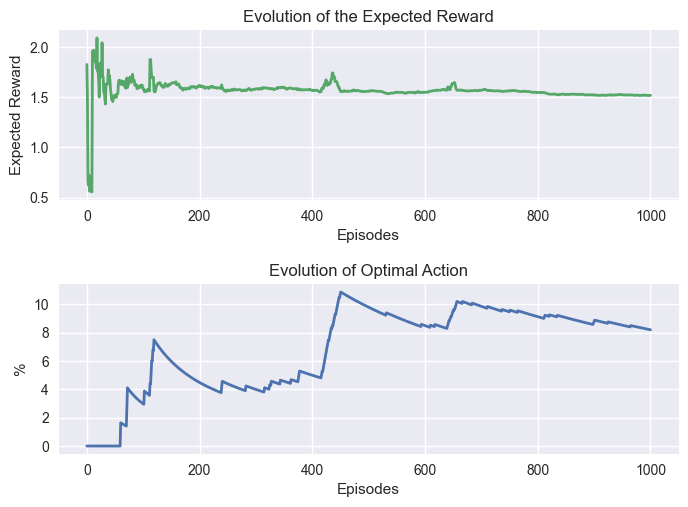
Two things is hapenning with these graphs:
The expected reward varied a lot at the beginning, but stabilize quickly.
The percentage of optimal action stabilized after a few hundred steps.