Let’s practice

We will see a very simple grid world problem. In this environment the agent start always in the same position and needs to reach a cell in the world. To complicate things for the agent, one cell is a trap and if the agent go on it the game is lost.

Visually the world will look like this:

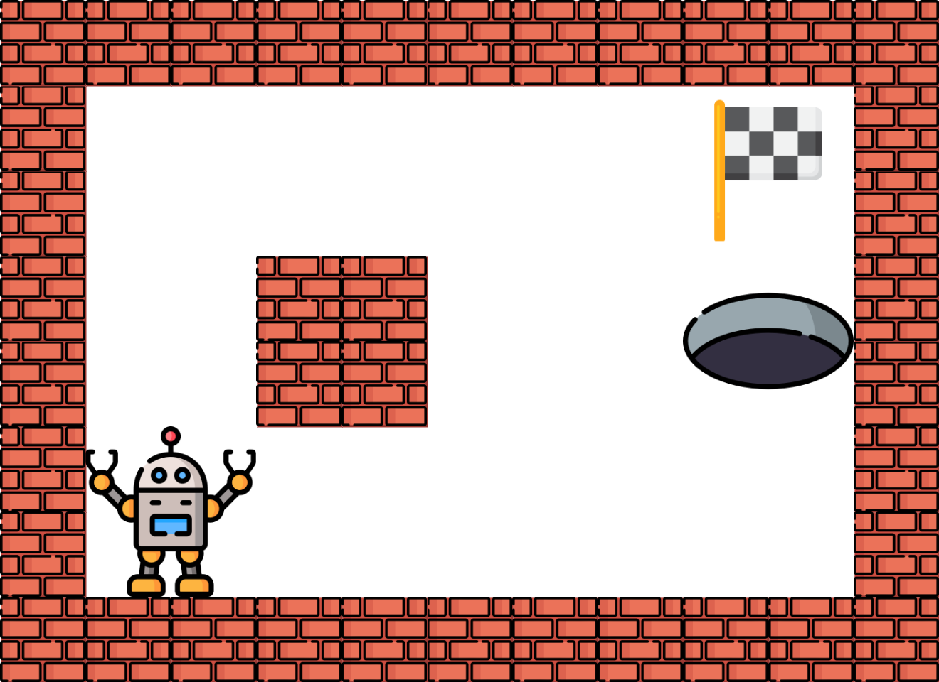
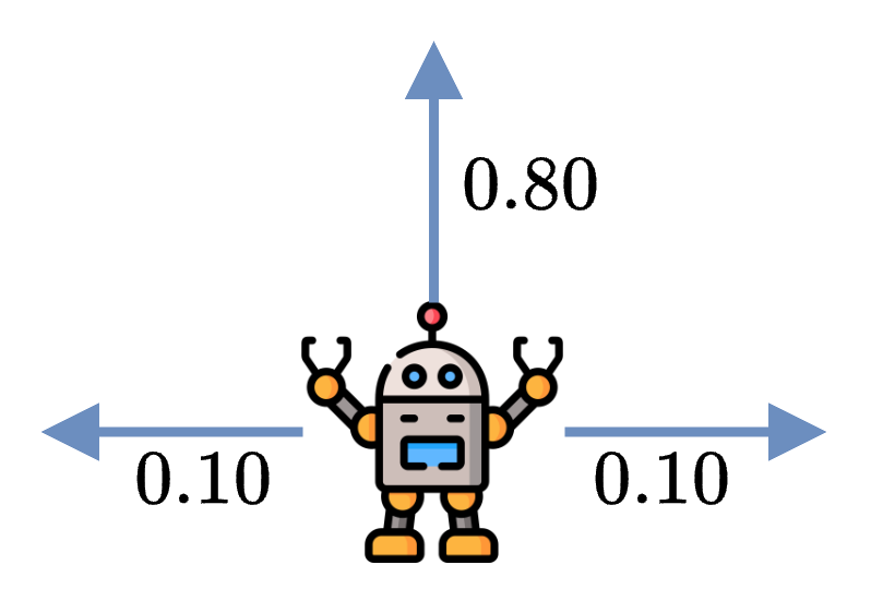
Since MDPs (Markov Decision Processes) are designed to solve stochastic problems, we will introduce some stochasticity to the problem. Specifically, we will add uncertainty to the agent’s movements. When the agent decides to move in one direction, such as UP, there is an 80% chance of moving in the desired direction and a 10% chance of moving to one of the adjacent cells.

If the agent moves into a wall, the agent stays in the same cell instead.

Markov Decision Process

Before implementing the environment and solving it, we need to define it as a MDP \(\Omega = (S,A,T,R)\), where:

• \(S\) is the state space: each state \(s\) will be a cell of the grid such as \(\forall s \in S, s \in [0, 11]\).

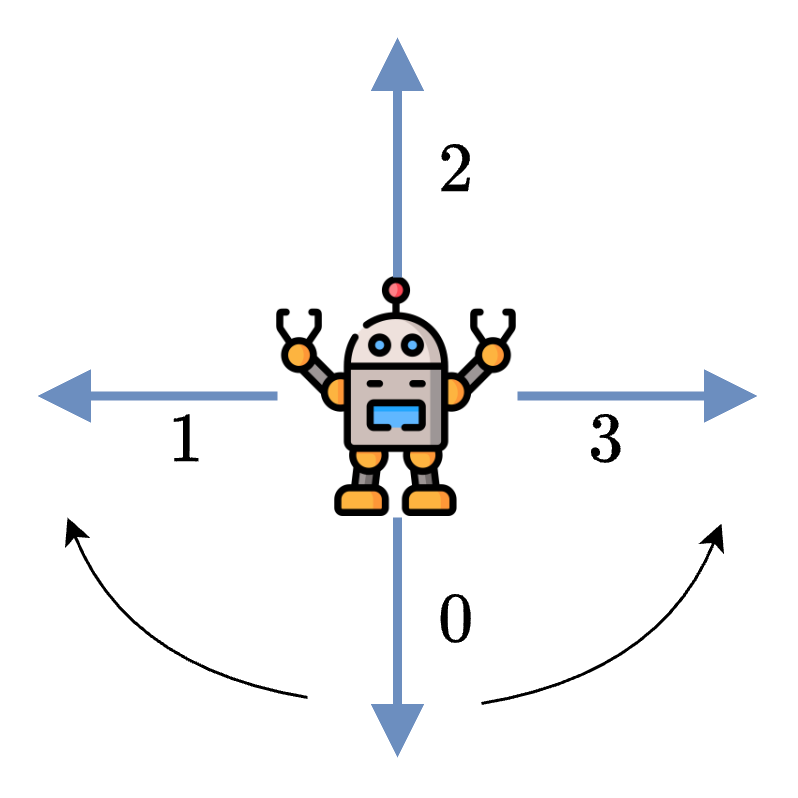
• \(A\) is the action space: each action \(a\) will be a direction such as \(\forall a \in A, a \in \{UP, DOWN, LEFT, RIGHT\}\).

• \(T\) is the transition function. Moving in a specific direction have a success chance of \(80\%\), and there is a \(20\%\) probability of going in the adjacent cells instead.

• \(R\) is the reward function: Entering the goal gives \(+10\), falling in the trap gives \(-10\), and all the other actions give \(0\).

Environment Implementation

Again, we will implement the environment using Gym conventions and call it GridWorld.

class GridWorld(gymnasium.Env):
  def __init__(self):
    pass

  def step(self, action: int):
    pass

State space and Action space

Based on our definition of the MDP, the state space represents all the states possible, which in this problem is all the cells the agent can reach, and the action space is all the action the agent can perform.

In both cases the spaces are discrete, so we can use the Discrete type of Gym to represent them.

self.action_space = spaces.Discrete(4) # Up, Down, Left, Right
self.observation_space = spaces.Discrete(12) # 12 cells

State space

There is not one way to represent the state space for a problem. In this problem we could represent it by the grid itself where the agent will be represented by the cell having boolean equal to True. You would have spaces.MultiDiscrete(np.array([3, 4])).

Note

We consider a state space containing 12 states, so it includes the wall cell. The agent cannot technically go on it, but it eases the implementation so we include it.

Transition function

In reinforcement learning, we don’t need to explicitly implement the transition function. However, solving MDPs with value iteration requires it:

\[V(s_{k+1}) = \sum_a\pi(a|s)\sum_{s'}p(s'|s,a)\left[ r(s,a) + \gamma v_k(s') \right]\]

Gym doesn’t provide any method or convention of doing it, so we’ll create a variable P representing our transition function. It will be a dictionary of dictionaries, where the first key is the current state and the second key will be the action. It will return the list of list containing the probability, the state and the reward.

self.P = { 0: { 0: [[0.9, 0, 0], [0.1, 1, 0]], 1: [[0.8, 4, 0], [0.1, 1, 0], [0.1, 0, 0]], 2: [[0.9, 0, 0], [0.1, 4, 0]], 3: [[0.8, 1, 0], [0.1, 4, 0], [0.1, 0, 0]]},
               1: { 0: [[0.8, 1, 0], [0.1, 0, 0], [0.1, 2, 0]],  1: [[0.8, 1, 0], [0.1, 0, 0], [0.1, 2, 0]], 2: [[0.8, 0, 0], [0.2, 1, 0]], 3: [[0.8, 2, 0], [0.2, 1, 0]]},
               2: { 0: [[0.8, 2, 0], [0.1, 1, 0], [0.1, 3, 0]], 1: [[0.8, 6, 0], [0.1, 1, 0], [0.1, 3, 0]], 2: [[0.8, 1, 0], [0.1, 2, 0], [0.1, 6, 0]], 3: [[0.8, 3, 0], [0.1, 2, 0], [0.1, 6, 0]]},
               3: { 0: [[0.9, 3, 0], [0.1, 2, 0]], 1: [[0.8, 7, -10], [0.1, 2, 0], [0.1, 3, 0]], 2: [[0.8, 2, 0], [0.1, 3, 0], [0.1, 7, -10]], 3: [[0.9, 3, 0], [0.1, 7, -10]]},
               4: { 0: [[0.8, 0, 0], [0.2, 4, 0]], 1: [[0.8, 8, 0], [0.2, 4, 0]], 2: [[0.8, 4, 0], [0.1, 0, 0], [0.1, 8, 0]], 3: [[0.8, 4, 0], [0.1, 0, 0], [0.1, 8, 0]]},
               5: { 0: [[1, 5, 0]], 1: [[1, 5, 0]], 2: [[1, 5, 0]], 3: [[1, 5, 0]]},
               6: { 0: [[0.8, 2, 0], [0.1, 6, 0], [0.1, 7, -10]], 1: [[0.8, 10, 0], [0.1, 6, 0], [0.1, 7, -10]], 2: [[0.8, 6, 0], [0.1, 10, 0], [0.1, 2, 0]], 3: [[0.8, 7, -10], [0.1, 2, 0], [0.1, 10, 0]]},
               7: { 0: [[1, 7, -10]], 1: [[1, 7, -10]], 2: [[1, 7, -10]], 3: [[1, 7, -10]]},
               8: { 0: [[0.8, 4, 0], [0.1, 9, 0], [0.1, 8, 0]], 1: [[0.9, 8, 0], [0.1, 9, 0]], 2: [[0.9, 8, 0], [0.1, 4, 0]], 3: [[0.8, 9, 0], [0.1, 4, 0], [0.1, 8, 0]]},
               9: { 0: [[0.8, 9, 0], [0.1, 8, 0], [0.1, 10, 0]], 1: [[0.8, 9, 0], [0.1, 8, 0], [0.1, 10, 0]], 2: [[0.8, 8, 0], [0.2, 9, 0]], 3: [[0.8, 10, 0], [0.2, 9, 0]]},
               10: { 0: [[0.8, 6, 0], [0.1, 9, 0], [0.1, 11, 10]], 1: [[0.8, 10, 0], [0.1, 9, 0], [0.1, 11, 10]], 2: [[0.8, 9, 0], [0.1, 6, 0], [0.1, 10, 0]], 3: [[0.8, 11, 10], [0.1, 6, 0], [0.1, 10, 0]]},
               11: { 0: [[1, 11, 10]], 1: [[1, 11, 10]], 2: [[1, 11, 10]], 3: [[1, 11, 10]]},
              } 

It is preferable to not use the variable P for applying the transition in the environment. We can implement it by modifying the action based on a random number to simulate the error. If the random number is below \(0.8\), then it is a success and the action stays the same. Otherwise the action is changed to the clockwise or counterclockwise action.

prob = np.random.random()
if prob < 0.80:
  actual_action = action
elif prob < 0.90:
  # Adjacent cell "clockwise"
  actual_action = (action + 1) % 4
else:
  # Adjacent cell "counterclockwise"
  actual_action = (action - 1) % 4  

Our state is represented as an integer, but we can convert it to coordinates.

r = np.floor(self.state / 3)
c = self.state % 4

Once it is done we can apply the action and modify the coordinates.

if actual_action == 0:
  r = max(0, r - 1)
elif actual_action == 2:
  r = min(2, r + 1)
elif actual_action == 1:
  c = max(0, c - 1)
elif actual_action == 3:
  c = min(3, c + 1)

And finally, we convert it back to an integer.

self.state = r * 4 + c

If we put everything together, we obtain a function that will manage the transition for us.

  def _transition(self, action: int):
    """
    Transition function.
    :param action: Action to take
    """
    r = np.floor(self.state / 3)
    c = self.state % 4

    prob = np.random.random()
    if prob < 0.80:
      actual_action = action
    elif prob < 0.90:
      # Adjacent cell "clockwise"
      actual_action = (action + 1) % 4
    else:
      # Adjacent cell "counterclockwise"
      actual_action = (action - 1) % 4


    if actual_action == 0:
      r = max(0, r - 1)
    elif actual_action == 2:
      r = min(2, r + 1)
    elif actual_action == 1:
      c = max(0, c - 1)
    elif actual_action == 3:
      c = min(3, c + 1)
    self.state = r * 4 + c

Reward function

The reward is straightforward, if we reach the \(+10\) (\(-10\)) cell the agent receive \(+10\) (\(-10\)), otherwise the rewards is always \(0\).

We implement the reward directly in the step function.

  def step(self, action: int):
    self._transition(action)
    
    done = False

    reward = 0
    if self.state == 11:
      reward = 10
      done = True
    elif self.state == 7:
      reward = -10
      done = True

    # Return the observation, reward, done flag, and info
    return self.state, reward, done, {}

Everything together

The full environment is provided below. You will see it contains a way to render the environment, it can be useful sometimes.

Activity

The function render doesn’t show the position of the agent and it is up to you to finish it.

Show code cell source Hide code cell source

import gymnasium
from gymnasium import spaces
import numpy as np
import matplotlib.pyplot as plt
from matplotlib.patches import Rectangle

class GridWorld(gymnasium.Env):
  def __init__(self):
    # Define the action and observation spaces
    self.action_space = spaces.Discrete(4) # Up, Down, Left, Right
    self.observation_space = spaces.Discrete(12) # 12 cells

    self.P = { 0: { 0: [[0.9, 0, 0], [0.1, 1, 0]], 1: [[0.8, 4, 0], [0.1, 1, 0], [0.1, 0, 0]], 2: [[0.9, 0, 0], [0.1, 4, 0]], 3: [[0.8, 1, 0], [0.1, 4, 0], [0.1, 0, 0]]},
               1: { 0: [[0.8, 1, 0], [0.1, 0, 0], [0.1, 2, 0]],  1: [[0.8, 1, 0], [0.1, 0, 0], [0.1, 2, 0]], 2: [[0.8, 0, 0], [0.2, 1, 0]], 3: [[0.8, 2, 0], [0.2, 1, 0]]},
               2: { 0: [[0.8, 2, 0], [0.1, 1, 0], [0.1, 3, 0]], 1: [[0.8, 6, 0], [0.1, 1, 0], [0.1, 3, 0]], 2: [[0.8, 1, 0], [0.1, 2, 0], [0.1, 6, 0]], 3: [[0.8, 3, 0], [0.1, 2, 0], [0.1, 6, 0]]},
               3: { 0: [[0.9, 3, 0], [0.1, 2, 0]], 1: [[0.8, 7, -10], [0.1, 2, 0], [0.1, 3, 0]], 2: [[0.8, 2, 0], [0.1, 3, 0], [0.1, 7, -10]], 3: [[0.9, 3, 0], [0.1, 7, -10]]},
               4: { 0: [[0.8, 0, 0], [0.2, 4, 0]], 1: [[0.8, 8, 0], [0.2, 4, 0]], 2: [[0.8, 4, 0], [0.1, 0, 0], [0.1, 8, 0]], 3: [[0.8, 4, 0], [0.1, 0, 0], [0.1, 8, 0]]},
               5: { 0: [[1, 5, 0]], 1: [[1, 5, 0]], 2: [[1, 5, 0]], 3: [[1, 5, 0]]},
               6: { 0: [[0.8, 2, 0], [0.1, 6, 0], [0.1, 7, -10]], 1: [[0.8, 10, 0], [0.1, 6, 0], [0.1, 7, -10]], 2: [[0.8, 6, 0], [0.1, 10, 0], [0.1, 2, 0]], 3: [[0.8, 7, -10], [0.1, 2, 0], [0.1, 10, 0]]},
               7: { 0: [[1, 7, -10]], 1: [[1, 7, -10]], 2: [[1, 7, -10]], 3: [[1, 7, -10]]},
               8: { 0: [[0.8, 4, 0], [0.1, 9, 0], [0.1, 8, 0]], 1: [[0.9, 8, 0], [0.1, 9, 0]], 2: [[0.9, 8, 0], [0.1, 4, 0]], 3: [[0.8, 9, 0], [0.1, 4, 0], [0.1, 8, 0]]},
               9: { 0: [[0.8, 9, 0], [0.1, 8, 0], [0.1, 10, 0]], 1: [[0.8, 9, 0], [0.1, 8, 0], [0.1, 10, 0]], 2: [[0.8, 8, 0], [0.2, 9, 0]], 3: [[0.8, 10, 0], [0.2, 9, 0]]},
               10: { 0: [[0.8, 6, 0], [0.1, 9, 0], [0.1, 11, 10]], 1: [[0.8, 10, 0], [0.1, 9, 0], [0.1, 11, 10]], 2: [[0.8, 9, 0], [0.1, 6, 0], [0.1, 10, 0]], 3: [[0.8, 11, 10], [0.1, 6, 0], [0.1, 10, 0]]},
               11: { 0: [[1, 11, 10]], 1: [[1, 11, 10]], 2: [[1, 11, 10]], 3: [[1, 11, 10]]},
              } 

    # Initialize the state
    self.state = 0

  def step(self, action: int):

    self._transition(action)

    done = False

    reward = 0
    if self.state == 11:
      reward = 10
      done = True
    elif self.state == 7:
      reward = -10
      done = True


    # Return the observation, reward, done flag, and info
    return self.state, reward, done, {}

  def _transition(self, action: int):
    """
    Transition function.
    :param action: Action to take
    """
    r = np.floor(self.state / 4)
    c = self.state % 3

    prob = np.random.random()
    if prob < 0.80:
      actual_action = action
    elif prob < 0.90:
      # Adjacent cell "clockwise"
      actual_action = (action + 1) % 4
    else:
      # Adjacent cell "counter clockwise"
      actual_action = (action - 1) % 4


    if actual_action == 0:
      r = max(0, r - 1)
    elif actual_action == 2:
      r = min(2, r + 1)
    elif actual_action == 1:
      c = max(0, c - 1)
    elif actual_action == 3:
      c = min(3, c + 1)
    self.state = r * 4 + c

  def reset(self):
    """
    Reset the environment.
    """
    self.state = 0
    return self.state

  def render(self, render="human"):
    fig, ax = plt.subplots()
    ax.set_xlim(0, 4)
    ax.set_ylim(0, 3)
    ax.set_aspect('equal')


    for i in range(4):
      for j in range(3):
        if j * 4 + i == 11:
          rect = Rectangle((i, j), 1, 1, edgecolor='black', facecolor='green')
          ax.add_patch(rect)
        elif j * 4 + i == 7:
          rect = Rectangle((i, j), 1, 1, edgecolor='black', facecolor='red')
          ax.add_patch(rect)
        elif j * 4 + i == 5:
          rect = Rectangle((i, j), 1, 1, edgecolor='black', facecolor='grey')
          ax.add_patch(rect)
        else:
          rect = Rectangle((i, j), 1, 1, edgecolor='black', facecolor='white')
          ax.add_patch(rect)

    ax.tick_params(axis='both',       # changes apply to both axis
                    which='both',      # both major and minor ticks are affected
                    bottom=False,      # ticks along the bottom edge are off
                    top=False,         # ticks along the top edge are off
                    left=False,
                    right=False,
                    labelbottom=False,
                    labelleft=False) # labels along the bottom edge are off

    plt.show()

Value Iteration

Value Iteration is very easy to implement, and take advantage of the information provide by the environment to simplify the code.

def value_iteration(env, gamma=0.9, theta=0.0001):
  V = np.zeros(env.observation_space.n)
  while True:
    delta = 0
    for s in range(env.observation_space.n):
      v = V[s]
      V[s] = max([sum([p * (r + gamma * V[s_]) for p, s_, r in env.P[s][a]]) for a in env.P[s]])
      delta = max(delta, np.abs(v - V[s]))
      V[7] = -10
      V[11] = 10
    if delta < theta:
      break
  pi = np.zeros(env.observation_space.n)
  for s in range(env.observation_space.n):
    pi[s] = np.argmax([sum([p * (r + gamma * V[s_]) for p, s_, r in env.P[s][a]]) for a in env.P[s]])
  return V, pi

We can use the observation space to intialize the value function with zeros.

V = np.zeros(env.observation_space.n)

We update the value for each state by looping other them (using the observation space again) and we apply the formula. This is where we actually need P, because it simplifies the code a lot.

V[s] = max([sum([p * (r + gamma * V[s_]) for p, s_, r in env.P[s][a]]) for a in env.P[s]])

Theta

The value of theta is up to you, but if theta is too big yo may not converge to the optimal policy. Too small, it could take a long time to converge.

Finally, once we converged (based on \(\theta\)) we calculate the policy the same way we calculated the value function but we use argmax instead.

for s in range(env.observation_space.n):
    pi[s] = np.argmax([sum([p * (r + gamma * V[s_]) for p, s_, r in env.P[s][a]]) for a in env.P[s]])

While we run the algorithm, we can observe the evolution of the value function for each state. Value Iteration being a dynamic programming algorithm, we see that the first state being updated is the one close to the goal. In the following steps, the states are being progressively updated until it converges.

Example

In the example the values are rounded to the nearest integers for rendering purposes.

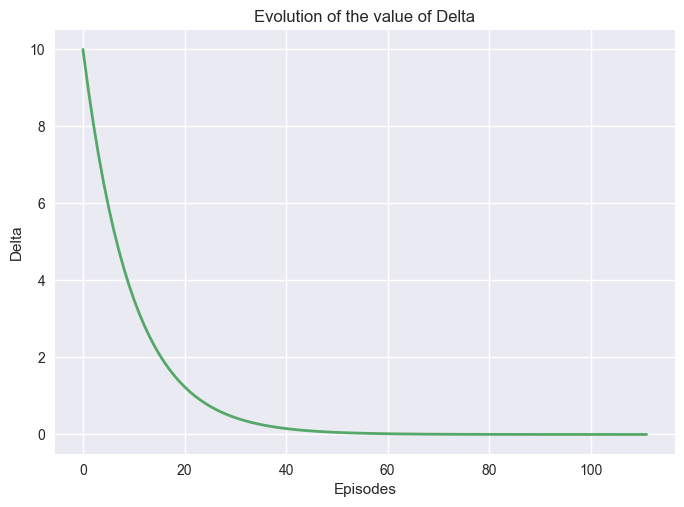
It is also possible to study how the value function convergences by plotting the value of \(\delta\).

Impact of the discount rate

If we are setting the discount rate to \(\gamma=0.5\) the algorithms converges quickly. However, it doesn’t mean it converges to the same policy or that the policy will perform similarly to the previous one.

import matplotlib.pyplot as plt

def plot_vi_conv(deltas):
    plt.style.use('seaborn-v0_8')
    x = np.linspace(0, len(deltas), len(deltas))

    fig, ax1= plt.subplots()
    plt.subplots_adjust(hspace=0.5)

    ax1.plot(x, deltas, linewidth=2.0, color="C1")
    ax1.set_title("Evolution of the value of Delta")
    ax1.set_ylabel("Delta")
    ax1.set_xlabel("Episodes")

    plt.show()

Important

Changing theta will increase or decrease the time it will take for the algorithm to stop, but it will impact the quality of the policy. If the algorithms stop too soon, meaning before it converges, the policy obtained could be suboptimal. However, larger problems can be too large to be calculated optimally, and a partial solution may be enough.

Interactive Visualizations

The following interactive visualizations help you explore the behavior of value iteration with different parameters.