Policies and Value Function

Now that we understand why we need systematic decision-making and evaluation tools, let’s formalize these concepts mathematically.

Policies tell us what to do in each situation, while value functions tell us how good each situation is. Together, they let us find optimal solutions to sequential decision problems.

Cumulative rewards

When making decisions, we care about more than just immediate rewards. We want to maximize the total reward we’ll receive over time.

• Remember that after few time steps we obtain a trajectory:

• Similarly we also obtain a sequence of rewards associated to this trajectory:

Since actions have lasting consequences, we need to consider which part of this reward sequence we want to maximize. This is complicated by the fact that for the same action in the same state, the next future state is not certain due to the stochastic nature of transitions.

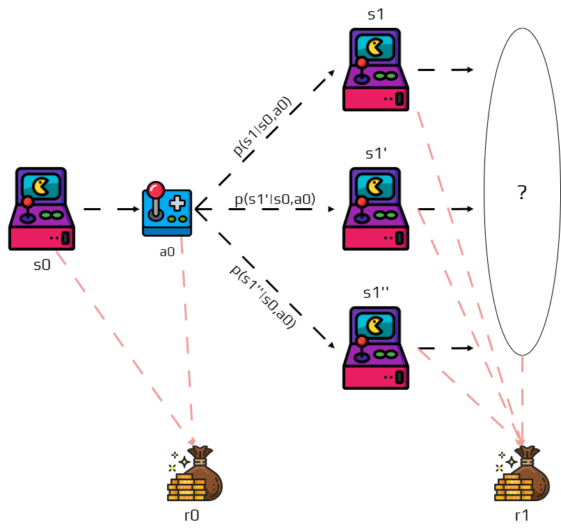
In reinforcement learning we try to maximize the expected return (average outcome across all possible futures). The return is denoted \(G_t\) and can be defined as the sum of the rewards:

\[ G_t = r_{t} + r_{t+1} + \dots + r_T \]

where \(T\) is the final step.

This definition is well-defined when \(T\) has a maximum value (finite episodes).

Example

• You receive three times a reward of \(10\).

• \(G_t\) is the sum of these rewards, so \(30\).

Activity

What happens if \(T=\infty\), meaning if the problem does not end?

When \(T=\infty\), the sum might blow up to infinity, making it impossible to compare different strategies. To address this, we introduce the notion of discounted return:

\[ G_t = r_{t} + \gamma r_{t+1} + \gamma^2 r_{t+2} = \sum_{k=0}^\infty \gamma^k r_{t+k} \]

where \(\gamma\) is a parameter \(0\leq\gamma\leq 1\) called discount rate.

The discount rate \(\gamma\) represents how much we value future rewards compared to immediate ones:

Discount rate

In most cases, the discount rate \(\gamma\) is around 0.9.

When \(\gamma = 0\), we only care about immediate rewards (completely myopic). When \(\gamma = 1\), future rewards are as important as immediate ones (completely farsighted). A typical value like \(\gamma = 0.9\) means future rewards matter, but less than immediate ones.

A reward received at step \(k\) is worth only \(\gamma^k\) times what it would be worth if received immediately. If \(\gamma = 0\), the agent is greedy, only considering immediate rewards. As \(\gamma\) approaches \(1\), the agent becomes more farsighted, planning further ahead.

Example

• You receive three times a reward of \(10\).

• But you apply a discount rate \(\gamma = 0.5\).

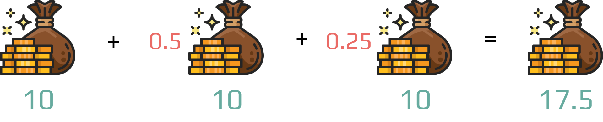
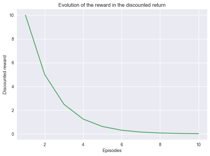
Following the same example, if we keep receiving a reward of \(10\) with a discount rate \(\gamma=0.5\). After \(10\) steps the discounted reward is close to \(0\).

import matplotlib.pyplot as plt
import numpy as np
from myst_nb import glue

G = []
for i in range(10):
  G.append(0.5**i * 10)

Impact of the discount rate

If we are setting the discount rate to \(\gamma=0.9\), later rewards are less discounted.

Note

Even if \(T=\infty\) the return is still finite

• if the reward is nonzero and constant and,

• if \(\gamma < 1\)

For example, if the reward is a constant \(+1\), then the return is:

\[ G_t = \sum_{k=0}^\infty \gamma^k = \frac{1}{1-\gamma} \]

Policies and Value functions

We know how to compute expected returns from reward sequences. Now we need to connect this to decision-making. Given that we’re in state \(s\), which action \(a\) should we choose to maximize our expected return?

We need two key tools: a policy (a systematic way to choose actions in each state) and a value function (a way to evaluate how good it is to be in each state). These work together—the value function evaluates how good a policy is, and we use this evaluation to improve the policy.

Definition 8 (Policy)

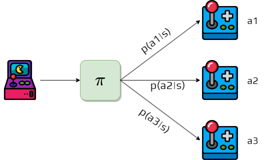
A policy is a mapping from states to probabilities of each possible action.

A policy \(\pi\) is like a “strategy manual” that tells the agent what to do in every possible situation. The notation \(\pi(a|s)\) represents the probability that the agent following policy \(\pi\) will select action \(a\) when in state \(s\).

Policies can be deterministic (always choosing the same action in a given state, with \(\pi(a|s) = 1\) for one action and \(0\) for others) or stochastic (choosing actions probabilistically, potentially selecting different actions in the same state).

For example, in a grid world, a policy might say “when in the top-left corner, move right with probability 0.7 and move down with probability 0.3.”

Definition 9 (Value function)

The value function of a state \(s\) under a policy \(\pi\) is the expected return when starting in \(s\) and following \(\pi\) thereafter.

The value function \(v_\pi(s)\) answers the question: “If I’m in state \(s\) and follow policy \(\pi\) from now on, what’s the expected total reward I’ll receive?” In MDPs, \(v_\pi\) is defined as:

\[ v_\pi(s) = \mathbb{E}_\pi\left[G_t | s_t=s \right] = \mathbb{E}_\pi\left[ \sum_{k=0}^\infty\gamma^k r_{t+k+1} | s_t = s \right] \]

This definition directly uses our return formula \(G_t\), connecting the concepts together. We use “expected” because due to stochastic transitions and policies, the actual return varies—the value function gives us the average return across all possible futures.

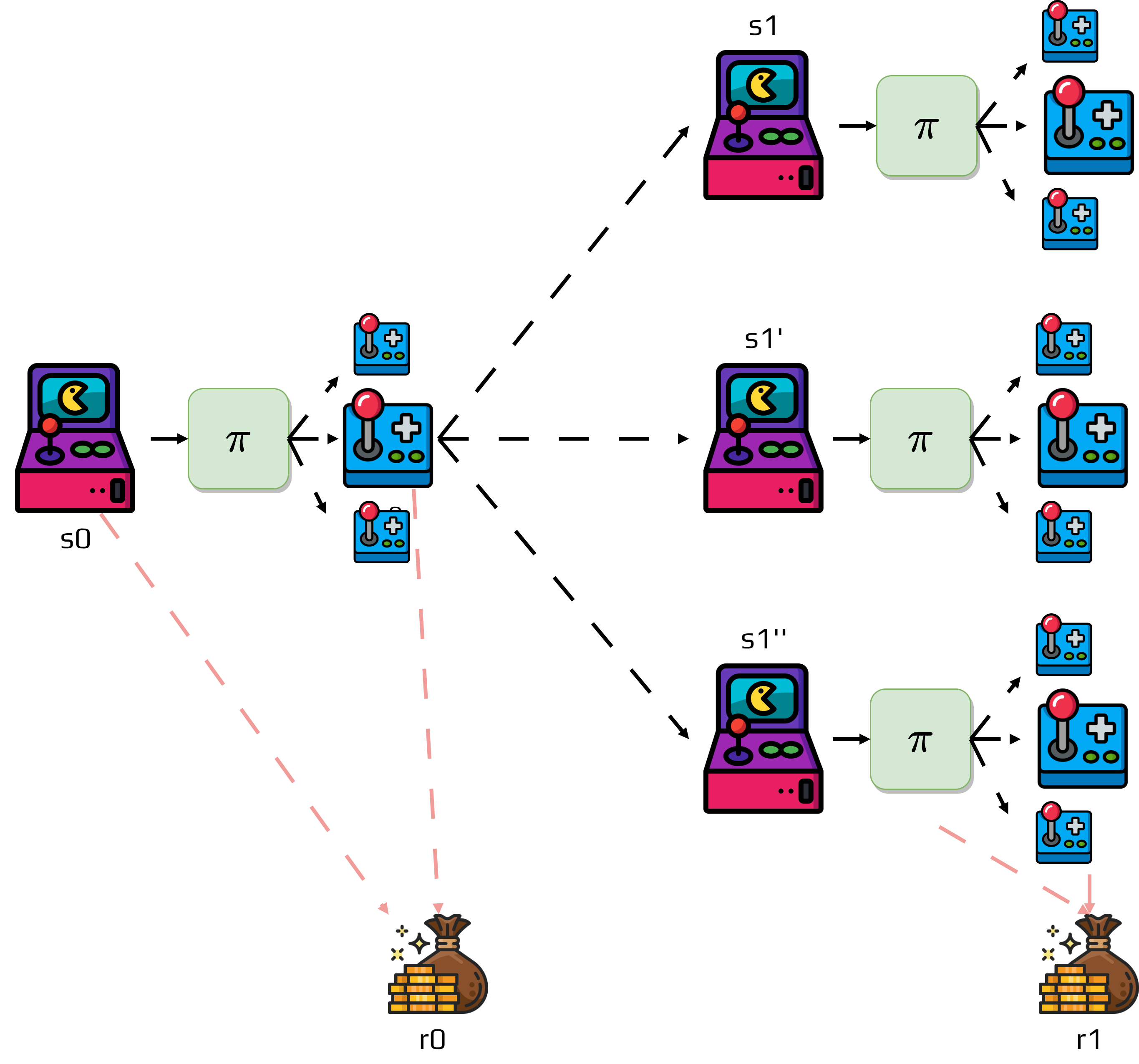
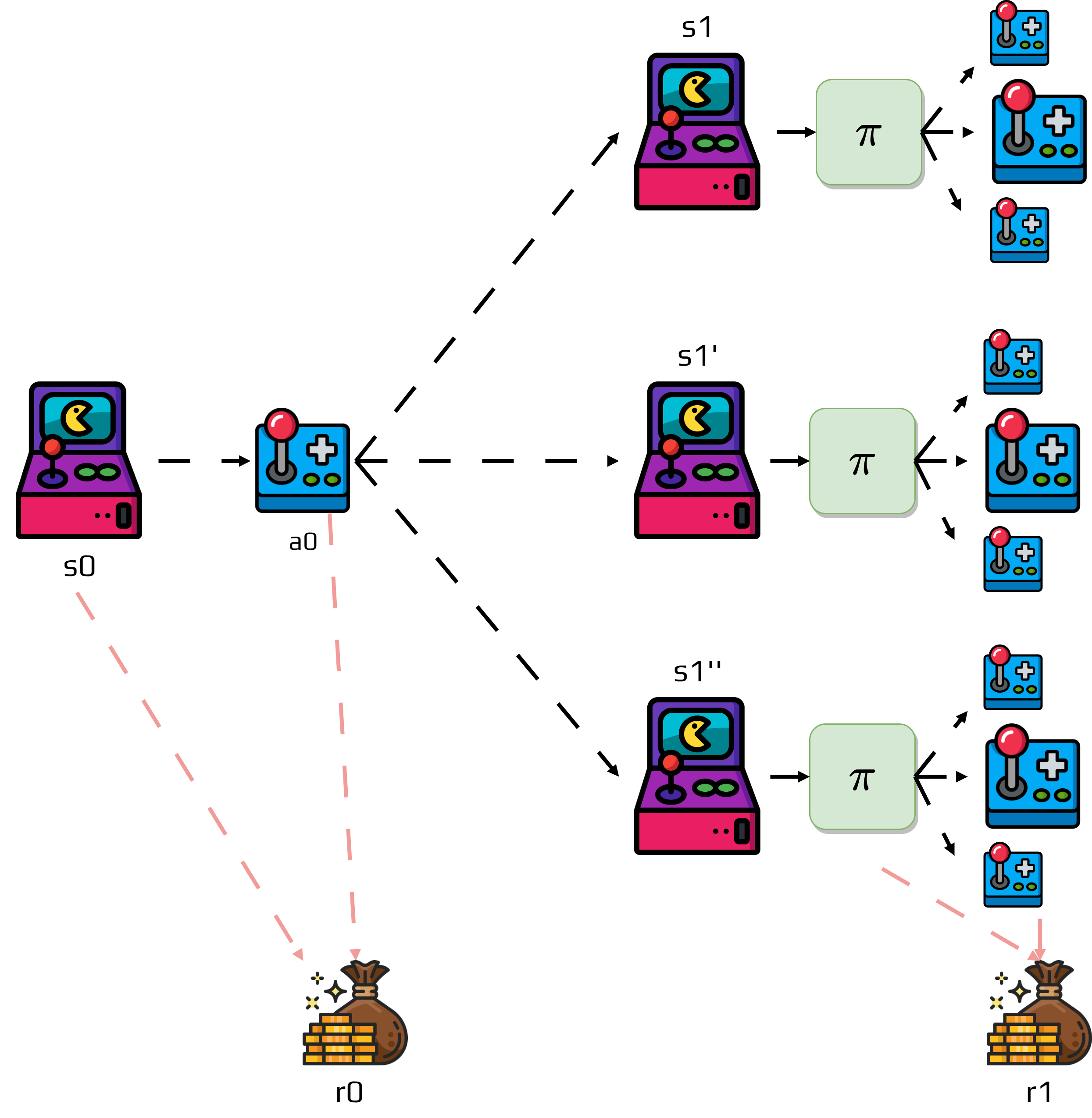
To calculate the expected return of state \(s_0\), we need to consider all possible trajectories and their probabilities:

Sometimes it’s useful to estimate the value of taking specific actions in a state. These are called q-values or action-value functions:

\[ q_\pi(s,a) = \mathbb{E}_\pi\left[G_t | s_t=s , a_t = a\right] = \mathbb{E}_\pi\left[ \sum_{k=0}^\infty\gamma^k r_{t+k+1} | s_t = s, a_t = a \right] \]

The function \(q_\pi(s,a)\) answers: “If I’m in state \(s\), take action \(a\), and then follow policy \(\pi\), what’s my expected return?” The state value is the expected action-value under the policy: $\(v_\pi(s) = \sum_a \pi(a|s) q_\pi(s,a)\)$

Q-values help us compare different actions in the same state to improve our policy.

Value functions have a crucial recursive property that makes them computable, known as the Bellman equation:

\[\begin{split} \begin{aligned} v_\pi(s) &= \mathbb{E}_\pi\left[G_t | s_t=s \right]\\ &= \mathbb{E}_\pi\left[r_{t} + \gamma G_{t+1}| s_t = s\right]\\ &= \sum_a \pi(a|s)\sum_{s'}p(s'|s,a)\left[ r(s,a) + \gamma\mathbb{E}_\pi\left[G_{t+1} | s_{t+1}=s' \right] \right]\\ &= \sum_a \pi(a|s)\sum_{s'}p(s'|s,a)\left[r + \gamma v_\pi(s')\right]\\ \end{aligned} \end{split}\]

This equation breaks down into immediate reward \(r(s,a)\) (what we get right now), future value \(\gamma v_\pi(s')\) (discounted value of where we end up), weighted by probabilities considering all possible actions and next states. This equation is powerful because it lets us compute values iteratively—if we know the values of future states, we can compute the current state’s value.

Bellman equation

The Bellman equation is dynamic programming applied to MDPs.

This is the Bellman equation for state values.

Optimal Policies and Optimal Value Functions

We can now calculate value functions for any given policy, but how do we find the best possible policy? Different policies will have different value functions, and we want to find the policy that gives us the highest values in all states.

Activity

Propose a method to calculate the optimal policy.

To determine which policy is better, we compare their value functions. Policy \(\pi\) is better than policy \(\pi'\) if: $\(v_\pi(s) \geq v_{\pi'}(s) \text{ for all states } s \in S\)$

A policy is better if it gives at least as much expected return from every possible starting state.

Important

Fundamental Theorem: There is always at least one policy that is better than or equal to all other policies.

The optimal policy, denoted \(\pi^*\), is the best possible policy for the MDP. The optimal value function, denoted \(v^*\), represents the best possible expected return from each state:

\[ v^*(s) = \max_\pi v_\pi(s), \forall s\in S \]

The function \(v^*(s)\) tells us “what’s the best possible expected return I can get if I start in state \(s\) and follow the optimal policy?”

Activity

Discuss if for the same MDP we can find more than one optimal policy.

Similarly, there’s an optimal action-value function:

\[ q^*(s,a) = \max_\pi q_\pi(s,a) \]

The optimal value function satisfies a special form of the Bellman equation called the Bellman optimality equation:

\[\begin{split} \begin{aligned} v^*(s) &= \max_{a\in A} q^*(s,a)\\ &= \max_a \mathbb{E}\left[ r_{t+1} + \gamma v^*(s_{t+1}) | s_t = s, a_t = a \right]\\ &= \max_a \sum_{s'}p(s'|s,a)\left[ r(s,a) + \gamma v^*(s') \right]\\ \end{aligned} \end{split}\]

Instead of averaging over the policy’s action probabilities, we take the maximum over all possible actions. The optimal value of a state equals the value of the best action we can take from that state.

Activity

What can you conclude from this equation?

Once we have the optimal value function \(v^*\), we can easily find the optimal policy:

\[ \pi^*(s) = \arg\max_a \sum_{s'}p(s'|s,a)\left[ r(s,a) + \gamma v^*(s') \right] \]

The process is straightforward: calculate \(v^*\) using the Bellman optimality equation, then choose actions that achieve the maximum in each state. This gives us the optimal policy that maximizes expected return. The optimal policy simply chooses the action that leads to the highest expected return from each state.