Assignment #1 - Tracking an Airplane
Worth: 10%
DUE: March 13th at 11:55pm; submitted on MOODLE.
Warning
For this assignment, you may not work with anyone else.
You need to work independently.
In this assignment you will solve your first nonlinear problem.
You will write a filter to track an airplane using a radar as a sensor.
2D problem
To stay simple, you will consider a 2D problem first:
The position relative to the ground
The altitude.
Problem modelisation
Radars work by emitting radio waves or microwaves. Anything in the beam’s path will reflect some of the signal back to the radar. By timing how long it takes for the reflected signal to return, it can compute the slant distance to the target.
Slant distance is the straight-line distance from the radar to the object. Bearing is computed using the directive gain of the antenna.
We compute the (x,y) position of the aircraft from the slant distance and elevation angle as illustrated by this diagram:
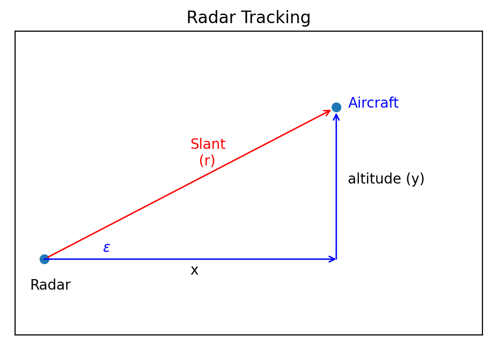
The elevation angle \(\epsilon\) is the angle above the line of sight formed by the ground.
You will assume that the aircraft is flying at the constant altitude. Thus we have a three variable state vector:
The state transition function is linear:
Implement the transition function:
def f_radar(x, dt):
    """ state transition function for a constant velocity
    aircraft with the state vector [distance, velocity, altitude]"""
After you need to design the measurement function. Remember that the measurement function converts the filter’s prior into a measurement.
You need to convert the position and velocity of the aircraft into elevation angle and range from the radar station.
You need to calculate the slant range and the elevation angle. It is not very hard it just basic trigonometry.
Implement the measurement function:
def h_radar(x, radar_pos):
"""Measurement function, return a list [slant_range, elevation_angle] """
Radar and Aircraft Simulator
Now you need to simulate the radar and the aircraft.
Implement the following two classes:
class RadarStation:

    def __init__(self, pos, range_std, elev_angle_std):
        pass


    def reading_of(self, ac_pos):
        """ Returns (range, elevation angle) to aircraft.
        Elevation angle is in radians.
        """


    def noisy_reading(self, ac_pos):
        """ Compute range and elevation angle to aircraft with
        simulated noise"""


class ACSim:
    def __init__(self, pos, vel, vel_std):


    def update(self, dt):
        """ Compute and returns next position. Incorporates
        random variation in velocity. """
Implementing the filter
Now you need to implement the UKF. Don’t worry it is something that you have already done before, just not in a class.
I am giving you the structure of the class:
class UKF:
    """
    Implements the Scaled Unscented Kalman filter (UKF).
    This filter scales the sigma points to avoid strong nonlinearities.

    Parameters
    ----------
    dim_x : int
        Number of state variables for the filter. For example, if
        you are tracking the position and velocity of an object in two
        dimensions, dim_x would be 4.
    dim_z : int
        Number of of measurement inputs. For example, if the sensor
        provides you with position in (x,y), dim_z would be 2.
        This is for convience, so everything is sized correctly on
        creation. If you are using multiple sensors the size of `z` can
        change based on the sensor. Just provide the appropriate hx function
    dt : float
        Time between steps in seconds.
    hx : function(x,**hx_args)
        Measurement function. Converts state vector x into a measurement
        vector of shape (dim_z).
    fx : function(x,dt,**fx_args)
        function that returns the state x transformed by the
        state transition function. dt is the time step in seconds.
    radar_pos: radar position

    Attributes
    ----------
    mu : numpy.array(dim_x)
        state estimate vector
    Sigma : numpy.array(dim_x, dim_x)
        covariance estimate matrix
    mup : numpy.array(dim_x)
        Prior (predicted) state estimate. The *_prior and *_post attributes
        are for convienence; they store the  prior and posterior of the
        current epoch. Read Only.
    Sigmap : numpy.array(dim_x, dim_x)
        Prior (predicted) state covariance matrix. Read Only.
    z : ndarray
        Last measurement used in update(). Read only.
    Q : numpy.array(dim_z, dim_z)
        measurement noise matrix
    R : numpy.array(dim_x, dim_x)
        process noise matrix
    K : numpy.array
        Kalman gain
    y : numpy.array
        innovation residual
    """

    def __init__(self, dim_x, dim_z, dt, hx, fx, radar_pos):
        """
        Create a Kalman filter. You are responsible for setting the
        various state variables to reasonable values; the defaults below will
        not give you a functional filter.
        """


    def predict(self):
        """ Performs the predict step of the UKF. On return,
        self.mup and self.Sigmap contain the predicted state (mu)
        and covariance (Sigma). 'p' stands for prediction.
        """


    def update(self, z):


    def MerweWeightSigmaPoints(self, alpha=.1, beta=2., kappa=0.):


    def SigmaPoints(self):


    def unscented_transform(self, sigmas, cov):
After that you need to execute the following code:
import math
import random
dt = 3. # 12 seconds between readings
range_std = 5 # meters
elevation_angle_std = math.radians(0.5)
ac_pos = (0., 1000.)
ac_vel = (100., 0.)
radar_pos = (0., 0.)
kf = UKF(3, 2, dt, fx=f_radar, hx=h_radar, radar_pos=radar_pos)
kf.R[0:2, 0:2] = np.array([[2.025, 1.35 ], [1.35 , 0.9 ]])
kf.R[2,2] = 0.1
kf.Q = np.diag([range_std**2, elevation_angle_std**2])
kf.mu = np.array([0., 90., 1000.])
kf.Sigma = np.diag([300**2, 30**2, 150**2])
np.random.seed(200)
pos = (0, 0)
radar = RadarStation(pos, range_std, elevation_angle_std)
ac = ACSim(ac_pos, (100, 0), 0.02)
time = np.arange(0, 360 + dt, dt)
xs = []
for _ in time:
ac.update(dt)
r = radar.noisy_reading(ac.pos)
kf.predict()
kf.update([r[0], r[1]])
xs.append(kf.mu)
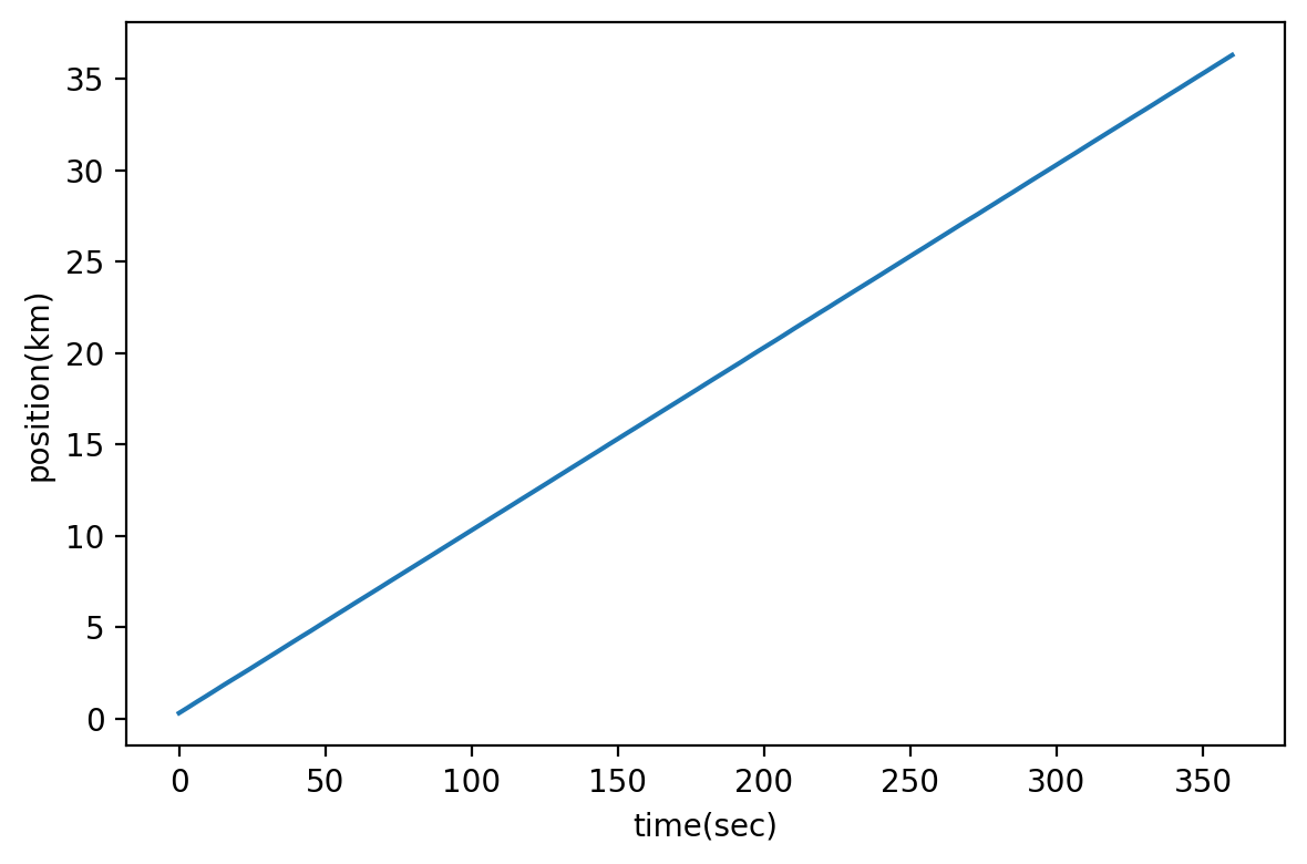
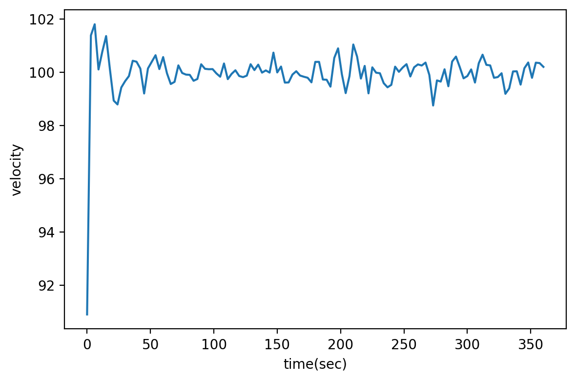
plot_radar(xs, time)
If everything is correct you should obtain something similar:
Tracking Maneuvering Aircraft
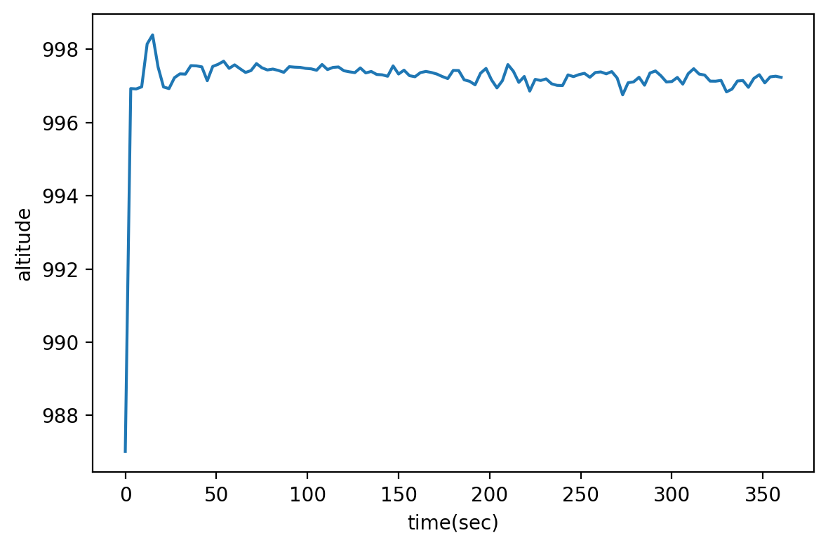
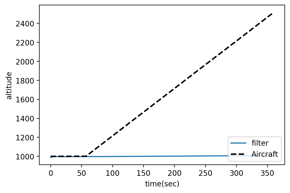
If you look at the results the filter is working very well, but we assumed that the airplane is not changing altitude.
If we apply the same filter with an airplane that is climbing, we obtain the following:
kf.x = np.array([0., 90., 1100.])
kf.P = np.diag([300**2, 30**2, 150**2])
ac = ACSim(ac_pos, (100, 0), 0.02)

np.random.seed(200)
time = np.arange(0, 360 + dt, dt)
xs, ys = [], []
for t in time:
    if t >= 60:
        ac.vel[1] = 300/60 # 300 meters/minute climb
    ac.update(dt)
    r = radar.noisy_reading(ac.pos)
    ys.append(ac.pos[1])
    kf.predict()
    kf.update([r[0], r[1]])
    xs.append(kf.mu)

plot_altitude(xs, time, ys)
The state and the transition function need to be changed to take into account the climbing rate:
Implement the new transition function:
def f_cv_radar(x, dt):
    """ state transition function for a constant velocity
    aircraft"""
You need to adapt the filter:
def cv_UKF(fx, hx, Q_std):
    # Implement the function here...
    return kf
First create a UKF
Secondly set R to the correct value (provided below)
Then, you need to create Q. Remember that you only have a float representing the std, but you want the variance as a matrix.
Set \(\mu\) and \(\Sigma\) (provided below)
kf.R[0:2, 0:2] = np.array([[2.025, 1.35 ], [1.35 , 0.9  ]])
kf.R[2:4, 2:4] = np.array([[2.025, 1.35 ], [1.35 , 0.9  ]])

mu = np.array([0., 90., 1000., 0.])
Sigma = np.diag([300**2, 3**2, 150**2, 3**2])
Now you can test it with the following code:
np.random.seed(200)
ac = ACSim(ac_pos, (100, 0), 0.02)
kf_cv = cv_UKF(f_cv_radar, h_radar, R_std=[range_std, elevation_angle_std])
time = np.arange(0, 360 + dt, dt)
xs, ys = [], []
for t in time:
if t >= 60:
ac.vel[1] = 300/60 # 300 meters/minute climb
ac.update(dt)
r = radar.noisy_reading(ac.pos)
ys.append(ac.pos[1])
kf_cv.predict()
kf_cv.update([r[0], r[1]])
xs.append(kf_cv.mu)
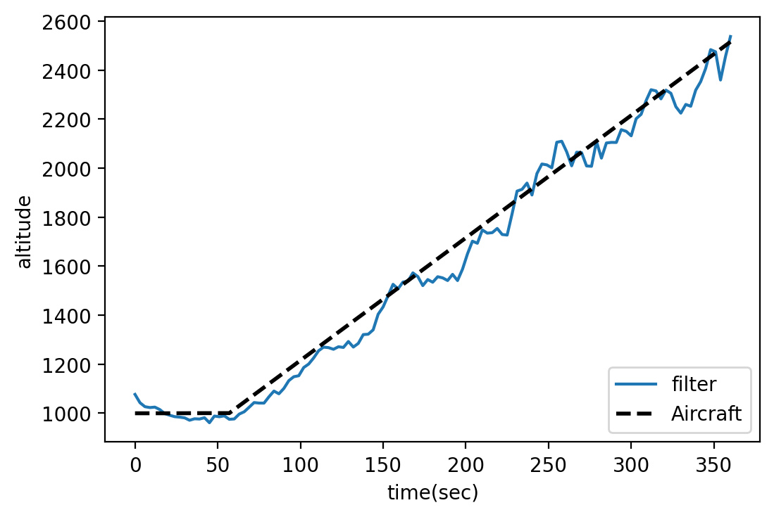
plot_altitude(xs, time, ys)
You should obtain something similar:
How to submit your work
You need to submit your unique python (.py) file directly on moodle. The first two lines of the python file should be as follows:
# Student name:
# Student number: