Topic 5 - Gaussian filters
Introduction
We will talk about one of the most important types of filters, the Gaussian filters.
Historically, Gaussian filters constitute the earliest tractable of the Bayes filter for continuous spaces.
Key idea
Gaussian techniques all share the idea that beliefs are represented by multivariate normal distributions.
The most studied technique is the Kalman Filter (KF). It is a technique for filtering and prediction in linear Gaussian systems.
The KF represents beliefs by the moment parameterization:
At time \(t\) is represented by the mean \(\mu_t\),
and the covariance \(\Sigma_t\).
Posteriors are Gaussian if and only if:
The state transition probability \(p(x_t|u_t,x_{t-1})\) is a linear function with added Gaussian noise.
The measurement probability \(p(z_t|x_t)\) is also linear in its argument with added Gaussian noise.
Before going further into the details, we will give the intuition with an example.
Problem definition
As for the Discrete Bayes Filter, we will be tracking a moving object in a long hallway at work.
We have a tracker that provides a reasonably accurate position of the dog.
The sensor returns the distance of the dog from the left end of the hallway in metres.
The sensor is not perfect. A reading of 23.4 could correspond to the dog being at 23.7, or 23.0.
However, it is very unlikely to correspond to a position of 47.6.
Furthermore, the errors seemed to be evenly distributed on both sides of the true position.
We predict that the dog is moving.
This prediction is not perfect.
Sometimes our prediction will overshoot, sometimes it will undershoot.
We are more likely to undershoot or overshoot by a little than a lot. Perhaps we can also model this with a Gaussian.
One-dimensional Kalman filter
Belief as Gaussians
We can express our belief in the dog’s position with a Gaussian.
Say we believe that our dog is at 10 metres, and the variance in that belief is 1 \(m^2\), or \(\mathcal{N}(10,\, 1)\).
A plot of the pdf follows
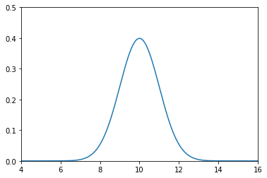
This plot depicts our uncertainty about the dog’s position.
It represents a fairly inexact belief. While we believe that it is most likely that the dog is at 10 m, any position from 9 m to 11 m or so are quite likely as well.
Assume the dog is standing still, and we query the sensor again. This time it returns 10.2 m.
Activity
Can we use this additional information to improve our estimate?
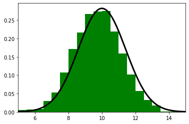
Consider: if we read the sensor 500 times and each time it returned a value between 8 and 12, all centered around 10, we should be very confident that the dog is near 10.
Of course, a different interpretation is possible. Perhaps our dog was randomly wandering back and forth in a way that exactly emulated random draws from a normal distribution. But that seems extremely unlikely - I’ve never seen a dog do that.
Let’s look at 500 draws from \(\mathcal N(10, 1)\):
import numpy as np
from numpy.random import randn
import matplotlib.pyplot as plt

xs = range(500)
ys = randn(500)*1. + 10.
plt.plot(xs, ys)
print(f'Mean of readings is {np.mean(ys):.3f}')
Mean of readings is 10.001
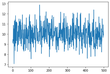
No dog moves like this.
However, noisy sensor data certainly looks this way.
Assuming the dog is standing still, we say the dog is at position 10 with a variance of 1.
Tracking with Gaussian Probabilities
If you remember the discrete Bayes filter, we used a histogram of probabilities to track the dog.
Each bin in the histogram represents a position, and the value is the probability of the dog in that position.
We used the equations:
We can replace \(\mathbf{x}\) by a Gaussian.
Important
We can replace hundreds to thousands of numbers with a single pair of numbers: \(x = \mathcal N(\mu, \sigma^2)\).
In this case, we obtain the following equations:
Predictions with Gaussians
We use Newton’s equation of motion to compute current position based on the current velocity and previous position:
I’ve dropped the notation \(f_x(\bullet)\) in favour of \(f_x\) to keep the equations uncluttered.
If the dog is at 10 m, his velocity is 15 m/s, and the epoch is 2 seconds long, we have
We are uncertain about his current position and velocity, so this will not do. We need to express the uncertainty with a Gaussian.
Position is easy. We define \(x\) as a Gaussian. If we think the dog is at 10 m, and the standard deviation of our uncertainty is 0.2 m, we get \(x=\mathcal N(10, 0.2^2)\).
What about our uncertainty in his movement? We define \(f_x\) as a Gaussian. If the dog’s velocity is 15 m/s, the epoch is 1 second, and the standard deviation of our uncertainty is 0.7 m/s, we get \(f_x = \mathcal N (15, 0.7^2)\).
The equation for the prior is
Remember that we can add two gaussians. Thus, we get:
We can implement this in python.
from collections import namedtuple
gaussian = namedtuple('Gaussian', ['mean', 'var'])
gaussian.__repr__ = lambda s: '𝒩(μ={:.3f}, 𝜎²={:.3f})'.format(s[0], s[1])
Now we can create and print a gaussian.
g1 = gaussian(3.4, 10.1)
g2 = gaussian(mean=4.5, var=0.2**2)
print(g1)
print(g2)
𝒩(μ=3.400, 𝜎²=10.100)
𝒩(μ=4.500, 𝜎²=0.040)
Here is our implementation of the predict function, where pos and movement are Gaussian tuples in the form \((\mu, \sigma^2)\):
def predict(pos, movement):
    return gaussian(pos.mean + movement.mean, pos.var + movement.var)
Let’s test it. What is the prior if the initial position is the Gaussian \(\mathcal N(10, 0.2^2)\) and the movement is the Gaussian \(\mathcal N (15, 0.7^2)\)?
pos = gaussian(10., .2**2)
move = gaussian(15., .7**2)
predict(pos, move)
𝒩(μ=25.000, 𝜎²=0.530)
The prior states that the dog is at 25 m with a variance of 0.53 \(m^2\), which is what we computed by hand.
Updates with Gaussians
Reminder
The discrete Bayes filter encodes our belief about the position of our dog in a histogram of probabilities.
The distribution is discrete and multimodal. It can express strong belief that the dog is in two positions at once, and the positions are discrete.
We are proposing that we replace the histogram with a Gaussian. The discrete Bayes filter used this code to compute the posterior:
def normalize(belief):
    return belief / sum(belief)

def update(likelihood, prior):
    return normalize(likelihood * prior)
We’ve just shown that we can represent the prior with a Gaussian.
The likelihood is the probability of the measurement given the current state.
For example, maybe our sensor states that the dog is at 23 m, with a standard deviation of 0.4 metres.
Our measurement, expressed as likelihood, is \(z = \mathcal N (23, 0.16)\).
Both the likelihood and prior are modelled with Gaussians.
Important
Can we multiply Gaussians? Is the product of two Gaussians another Gaussian?
Yes to the former, and almost to the latter! The product of two Gaussians is proportional to another Gaussian.
We can immediately infer several things.
If we normalize the result, the product is another Gaussian.
If one Gaussian is the likelihood, and the second is the prior, then the mean is a scaled sum of the prior and the measurement.
The variance is a combination of the variances of the prior and measurement.
Finally, the variances are completely unaffected by the values of the mean!
We put this in Bayesian terms like so:
If we implemented that in a function gaussian_multiply() we could implement our filter’s update step as
def gaussian_multiply(g1, g2):
    mean = (g1.var * g2.mean + g2.var * g1.mean) / (g1.var + g2.var)
    variance = (g1.var * g2.var) / (g1.var + g2.var)
    return gaussian(mean, variance)

def update(prior, likelihood):
    posterior = gaussian_multiply(likelihood, prior)
    return posterior
Activity
Implement the previous update function and test it with the following code.
predicted_pos = gaussian(10., .2**2)
measured_pos = gaussian(11., .1**2)
estimated_pos = update(predicted_pos, measured_pos)
estimated_pos
What is the estimated pos?
Play around and convince yourself that it’s working.
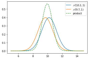
To convince ourselves we could plot the product of two gaussians.
def plot_products(g1, g2):
    plt.figure()
    product = gaussian_multiply(g1, g2)

    xs = np.arange(5, 15, 0.1)
    ys = [stats.gaussian(x, g1.mean, g1.var) for x in xs]
    plt.plot(xs, ys, label='$\mathcal{N}$'+'$({},{})$'.format(g1.mean, g1.var))

    ys = [stats.gaussian(x, g2.mean, g2.var) for x in xs]
    plt.plot(xs, ys, label='$\mathcal{N}$'+'$({},{})$'.format(g2.mean, g2.var))

    ys = [stats.gaussian(x, product.mean, product.var) for x in xs]
    plt.plot(xs, ys, label='product', ls='--')
    plt.legend()

z1 = gaussian(10.2, 1)
z2 = gaussian(9.7, 1)

plot_products(z1, z2)
First Kalman Filter
The kalman filter algorithm is very simple in a 1D problem:
def kalman_filter(x, zs):

    for z in zs:
        prior = predict(x, process_model)
        likelihood = gaussian(z, sensor_var)
        x = update(prior, likelihood)
Activity
Create a class DogSimulation that wil take as parameters:
The initial position
x0The velocity
velocityThe measurement variance
measurement_varThe process variance
process_var
The class needs to have a method move_and_sense() that will make the dog move and return the new measurement.
Implement the class and user it on the following example:
process_var = 1. # variance in the dog's movement
sensor_var = 2. # variance in the sensor

x = gaussian(0., 20.**2)  # dog's position, N(0, 20**2)
velocity = 1
dt = 1. # time step in seconds
process_model = gaussian(velocity*dt, process_var) # displacement to add to x

# simulate dog and get measurements
dog = DogSimulation(
    x0=x.mean,
    velocity=process_model.mean,
    measurement_var=sensor_var,
    process_var=process_model.var)

# create list of measurements
zs = [dog.move_and_sense() for _ in range(10)]
Graphically, we obtain something like this:
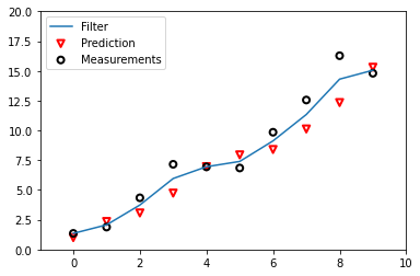
We can see the difference between the predictions and the measurements received. We also see what are the values returned by the filter.
Kalman Gain
We see that the filter works. Now let’s go back to the math to understand what is happening.
The posterior \(x\) is computed as the likelihood times the prior \((\mathcal L \bar x)\), where both are Gaussians.
Therefore the mean of the posterior is given by:
I use the subscript \(z\) to denote the measurement. We can rewrite this as:
In this form it is easy to see that we are scaling the measurement and the prior by weights:
The weights sum to one because the denominator is a normalization term. We introduce a new term, \(K=W_1\), giving us:
where
\(K\) is the Kalman gain. It’s the crux of the Kalman filter. It is a scaling term that chooses a value partway between \(\mu_z\) and \(\bar\mu\).
Let’s work a few examples. If the measurement is nine times more accurate than the prior, then \(\bar\sigma^2 = 9\sigma_z^2\), and
Hence \(K = \frac 9 {10}\), and to form the posterior we take nine tenths of the measurement and one tenth of the prior.
If the measurement and prior are equally accurate, then \(\bar\sigma^2 = \sigma_z^2\) and
which is the average of the two means. It makes intuitive sense to take the average of two equally accurate values.
We can also express the variance in terms of the Kalman gain:
We can understand this by looking at this chart:
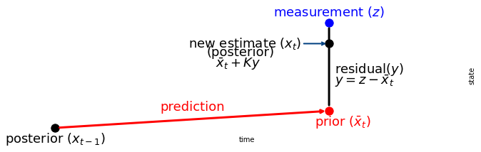
The Kalman gain \(K\) is a scale factor that chooses a value along the residual.
We can rewrite update() and predict() in function of the Kalman gain.
def update(prior, measurement):
    x, P = prior        # mean and variance of prior
    z, R = measurement  # mean and variance of measurement

    y = z - x        # residual
    K = P / (P + R)  # Kalman gain

    x = x + K*y      # posterior
    P = (1 - K) * P  # posterior variance
    return gaussian(x, P)

def predict(posterior, movement):
    x, P = posterior # mean and variance of posterior
    dx, Q = movement # mean and variance of movement
    x = x + dx
    P = P + Q
    return gaussian(x, P)
Important
This representation is the one used in the literature!
It is very important to understand it, and I will always refer to this notation.
This is extremely important to understand: Every filter in this course implements the same algorithm, just with different mathematical details.
The math can become challenging in later chapters, but the idea is easy to understand.
Here is the generic algorithm:
Initialization
Initialize the state of the filter
Initialize our belief in the state
Predict
Use system behavior to predict state at the next time step
Adjust belief to account for the uncertainty in prediction
Update
Get a measurement and associated belief about its accuracy
Compute residual between estimated state and measurement
Compute scaling factor based on whether the measurement or prediction is more accurate
Set state between the prediction and measurement based on scaling factor
Update belief in the state based on how certain we are in the measurement.
Equations for univariate Kalman Filter
The equations for the univariate Kalman filter are:
Predict
Update
Multivariate Kalman Filters
We implemented a Kalman filter for a problem in one dimension.
This is good and all, but one dimension is not enough in most robotic problems.
We need to have a way to implement it for two or more dimensions. We want a way to represent the position and velocity of a dog in a field.
Position and velocity are related to each other, and we should never throw away information.
Multivariate Normal Distributions
Until now, we used Gaussians for a scalar random variable, expressed as \(\mathcal{N}(\mu, \sigma^2)\). The formal term is univariate normal normal distribution.
As the name says, it considers only one variable. What we would like is to incorporate multiple variables.
Warning
It doesn’t necessarily mean spatial dimension!
Imagine we want to track the position, the velocity and acceleration of an aircraft in \((x, y, z)\) that gives us a nine dimensional problem.
So we will simplify for now!
We will use our example with Alan, so a problem with two dimensions (Alan doesn’t fly, he’s a dog not a pigeon).
We can see that for \(N\) dimensions, we need \(N\) means, which we will arrange in a column matrix (vector) like so:
Let’s say we believe that \(x = 2\) and \(y = 17\). We would have
The next step is representing our variances. At first blush we might think we would also need \(N\) variances for \(N\) dimensions. We might want to say the variance for \(x\) is 10 and the variance for \(y\) is 4, like so.
Activity
Do you agree with this?
This is incomplete because it does not consider the more general case.
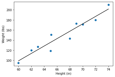
If we computed the variance in the heights of students. That is a measure of how the heights vary relative to each other.
If all students are the same height, then the variance is 0, and if their heights are wildly different, then the variance will be large.
There is also a relationship between height and weight. In general, a taller person weighs more than a shorter person.
Height and weight are correlated. We want a way to express not only what we think the variance is in the height and the weight, but also the degree to which they are correlated.
In other words, we want to know how weight varies compared to the heights. We call that the covariance.
Before we can understand multivariate normal distributions we need to understand the mathematics behind correlations and covariances.
Correlation and Covariance
Covariance describes how much two variables vary together.
Example
For example, as height increases weight also generally increases. These variables are correlated.
They are positively correlated because as one variable gets larger so does the other.
As the outdoor temperature decreases, home heating bills increase. These are inversely correlated or negatively correlated because as one variable gets larger the other variable lowers.
We will consider linear correlation, meaning that the relationship between variables is linear.
The equation for the covariance between \(X\) and \(Y\) is
Where \(\mathbb E[X]\) is the expected value of \(X\), defined as
We assume each data point is equally likely, so the probability of each is \(\frac{1}{N}\), giving
for the discrete case we will be considering.
Compare the covariance equation to the equation for the variance. As you can see they are very similar:
In particular, if you compute \(COV(X, X)\) you get the equation for \(VAR(X)\), which supports my statement that the variance computes how a random variable varies amongst itself.
We use a covariance matrix to denote covariances of a multivariate normal distribution, and it looks like this:
The diagonal contains the variance for each variable, and the off-diagonal elements contain the covariance between the \(i^{th}\) and \(j^{th}\) variables. So \(\sigma_3^2\) is the variance of the third variable, and \(\sigma_{13}\) is the covariance between the first and third variables.
A covariance of 0 indicates no correlation. If the variance for \(x\) is 10, the variance for \(y\) is 4, and there is no linear correlation between \(x\) and \(y\), then we would write
If there was a small amount of positive correlation between \(x\) and \(y\) we might have
where 1.2 is the covariance between \(x\) and \(y\). I say the correlation is “small” because the covariance of 1.2 is small relative to the variances of 10.
If there was a large amount of negative correlation between between \(x\) and \(y\) we might have
The covariance matrix is symmetric. After all, the covariance between \(x\) and \(y\) is always equal to the covariance between \(y\) and \(x\). That is, \(\sigma_{xy}=\sigma_{yx}\) for any \(x\) and \(y\).
Example
Suppose we have a class of students with heights \(H=[1.8, 2.0, 1.7, 1.9, 1.6]\) meters.
We can compute the variance:
Now, if we had their weights \(W=[70.1, 91.2, 59.5, 93.2, 53.5]\) in kg. We can use the covariance equation to calculate the covariance matrix:
We just computed the variance of the height, and it will go in the upper left-hand corner of the matrix. The lower right corner contains the variance in weights. Using the same equation we get:
Now the covariances. Using the formula above, we compute:
It is important to understand how this is calculated!
But we will not do that manually any longer, we will use NumPy to do that for us.
import numpy as np

W = [70.1, 91.2, 59.5, 93.2, 53.5]
H = [1.8, 2.0, 1.7, 1.9, 1.6]
np.cov(H, W)
array([[  0.025,   2.727],
       [  2.727, 327.235]])
NumPy applies a correction for small sample sizes. This is why we don’t obtain the same thing.
Multivariate Normal Distribution
Recall the equation for the normal distribution from the Gaussians chapter:
Here is the multivariate normal distribution in \(n\) dimensions.
The multivariate version merely replaces the scalars of the univariate equations with matrices.
We can plot a multivariate Gaussian with a mean \(\mu=[\begin{smallmatrix}2\\17\end{smallmatrix}]\) and a covariance of \(\Sigma=[\begin{smallmatrix}10&0\\0&4\end{smallmatrix}]\).
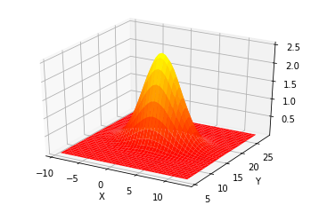
It shows the probability density for any value of \((X,Y)\) in the z-axis.
The curve for \(X\) is wider than the curve for \(Y\), which is explained by \(\sigma_x^2=10\) and \(\sigma_y^2=4\). The highest point of the 3D surface is at the the means for \(X\) and \(Y\).
Important
As with the univariate case this is a probability density, not a probability. Continuous distributions have an infinite range, and so the probability of being exactly at (2, 17), or any other point, is 0%.
We can compute the probability of being within a given range by computing the volume under the surface with an integral.
Now, we can wonder how it applies to our problem. Considering the following mean and covariance:
We can plot the error ellipses or confidence ellipses; the terms are interchangeable.
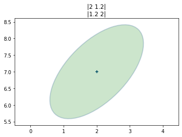
It plots the contour up to one standard deviation.
A Bayesian way of thinking about this is that the ellipse shows us the amount of error in our belief.
A tiny circle would indicate that we have a very small error, and a very large circle indicates a lot of error in our belief.
The shape of the ellipse shows us the geometric relationship of the errors in \(X\) and \(Y\).
A slanted ellipse tells us that the \(x\) and \(y\) values are somehow correlated. The off-diagonal elements in the covariance matrix are non-zero, indicating that a correlation exists.
Multiplying Multidimensional Gaussians
Multiplying multidimensional gaussians works in a similar fashion that with univariate gaussians.
The capital sigma (\(\Sigma\)) indicates that these are matrices, not scalars. Specifically, they are covariance matrices:
To give you some intuition about this, recall the equations for multiplying univariate Gaussians:
This looks similar to the equations for the multivariate equations. This will be more obvious if you recognize that matrix inversion, denoted by the -1 power, is like a reciprocal since \(AA^{-1} =I\).
I will rewrite the inversions as divisions - this is not a mathematically correct thing to do as division for matrices is not defined, but it does help us compare the equations.
In this form the relationship between the univariate and multivariate equations is clear.
Example
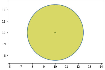
To illustrate this, consider a problem in which you want to track an airplane with two radar systems. (We consider a 2D problem.)
At first we are uncertain of the position of the aircraft, so the prior can be defined as:
Graphically it gives us:
Now suppose that there is a radar to the lower left of the aircraft.
Further suppose that the radar’s bearing measurement is accurate, but the range measurement is inaccurate.
We will consider the following covariance:
It might look like this (plotted in green on top of the yellow prior):
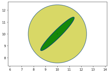
Recall that Bayesian statistics calls this the evidence.
The ellipse points towards the radar.
It is very long because the range measurement is inaccurate, and the aircraft could be within a considerable distance of the measured range.
It is very narrow because the bearing estimate is very accurate and thus the aircraft must be very close to the bearing estimate.
We want to find the posterior from incorporating the evidence into the prior.
If we use the previous mean and covariance:
I will not do the calcule manually we will use python and plot the result:

The posterior retained the same shape and position as the radar measurement, but is smaller.
We’ve seen this with one-dimensional Gaussians. Multiplying two Gaussians makes the variance smaller because we are incorporating more information, hence we are less uncertain.
Another point to recognize is that the covariance shape reflects the physical layout of the aircraft and the radar system. The importance of this will become clear in the next step.
Now we get a measurement from a second radar, this one to the lower right. The posterior from the last step becomes our new prior, which I plot in yellow.
The new measurement is plotted in green.
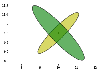
We incorporate this new measurement to calculate the posterior:
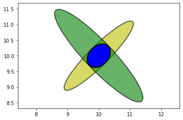
The only likely place for the aircraft is where the two ellipses intersect.
The intersection, formed by multiplying the prior and measurement, is a new Gaussian.
This allows us to triangulate on the aircraft, resulting in a very accurate estimate.
We didn’t explicitly write any code to perform triangulation; it was a natural outcome of multiplying the Gaussians of each measurement together.
Multivariate Kalman Filter
You’re now ready to implement the full form Kalman Filter.

We will be able to integrate the velocity of Alan in our estimation!
As always, we will limit ourselves to a specific subset of problems. The ones that can be described with Newton’s equation of motion.
These filters are called discretized continuous-time kinematic filters.
If we have time we will see the Kalman filter for non-Newtonian systems (maybe..).
Newton’s Equations of Motion
Newton’s equations of motion tells us that given a constant velocity \(v\) of a system we can compute its position \(x\) after time \(t\) with:
For example, if we start at position 13, our velocity is 10 m/s, and we travel for 12 seconds our final position is 133 (\(10\times 12 + 13\)).
We can incorporate constant acceleration with this equation
And if we assume constant jerk, we get
These equations were generated by integrating a differential equation.
Given a constant velocity \(v\) we can compute the distance travelled over time with the equation.
which we can derive with
To design a Kalman filter you need to start with a system of differential equations that describes the dynamics of the system.
Warning
Most systems of differential equations do not integrate easily in this way.
Newton’s equations are easy to integrate, this is why we only consider them for now.
Newton’s equations are the right equations to use to track moving objects, which is what we want.
Kalman Filter Algorithm
The algorithm is the same Bayesian filter algorithm that we have used in every chapter. The update step is slightly more complicated, but I will explain why when we get to it.
Pseudocode
Initialization
Initialize the state of the filter
Initialize our belief in the state
Predict
Use process model to predict state at the next time step
Adjust belief to account for the uncertainty in prediction.
Update
Get a measurement and associated belief about its accuracy
Compute residual between estimated state and measurement
Compute scaling factor based on whether the measurement or prediction is more accurate
set state between the prediction and measurement based on scaling factor
update belief in the state based on how certain we are in the measurement
As a reminder, here is a graphical depiction of the algorithm:
The univariate Kalman filter represented the state with a univariate Gaussian. Naturally, the multivariate Kalman filter will use a multivariate Gaussian for the state.
Equations for univariate Multivariate Kalman Filter
Predict
Without worrying about the specifics of the linear algebra, we can see that:
\(\mu,\, \Sigma\) are the state mean and covariance.
\(A\) is the state transition function. When multiplied by \(\mu\) it computes the prior.
\(R\) is the process covariance. It corresponds to \(\sigma^2_{f_x}\).
\(B\) and \(u\) are new to us. They let us model control inputs to the system.
Update
\(C\) is the measurement function. We haven’t seen this yet and I’ll explain it later. If you mentally remove \(C\) from the equations, you should be able to see these equations are similar as well.
\(z,\, Q\) are the measurement mean and noise covariance. They correspond to \(z\) and \(\sigma_z^2\) in the univariate filter.
\(y\) and \(K\) are the residual and Kalman gain.
The details will be different than the univariate filter because these are vectors and matrices, but the concepts are exactly the same:
Use a Gaussian to represent our estimate of the state and error
Use a Gaussian to represent the measurement and its error
Use a Gaussian to represent the process model
Use the process model to predict the next state (the prior)
Form an estimate part way between the measurement and the prior
Your job as a designer will be to design the state \(\left(x, \Sigma\right)\), the process \(\left(A, R\right)\), the measurement \(\left(z, Q\right)\), and the measurement function \(C\).
If the system has control inputs, such as a robot, you will also design \(B\) and \(u\).
The Kalman Filter Equations
Ok, at this poitn you might wonder that these equations are doing concretly.
That’s what we will see now.
Prediction Equations
The Kalman filter uses these equations to computer the prior, meaning the next state of the system.
We have the prior mean \(\bar \mu_t\) and the covariance \(\Sigma_t\).
As a reminder, the linear equation \(Ax = b\) represents a system of equations, where \(A\) holds the coefficients set of equations, \(x\) is the vector of variables.
Thus, if \(A\) contains the state transition for a given time step, then the product of \(A\mu\) computes the state after that transition.
Likewise, \(B\) is the control function, \(u\) is the control input, so \(Bu\) compute the contribution of the controls to the state after the transition.
Example
Consider \(A\) and \(\mu\):
Leading to \(\bar \mu = A\mu\) corresponds to the set of linear equations:
The equation of the covariance (\(\bar \Sigma = A \Sigma A^\mathsf T + R\)) is not easy to understand, so we will take some time to study it.
In univariate version of this equation is:
We add the variance of the movement to the variance of our estimate to reflect the loss of knowledge.
It isn’t quite that easy with multivariate Gaussians.
We can’t simply write \(\bar \Sigma = \Sigma + R\). In a multivariate Gaussians the state variables are correlated. What does this imply? Our knowledge of the velocity is imperfect, but we are adding it to the position with
Since we do not have perfect knowledge of the value of \(\dot x\) the sum \(\bar x = \dot x\Delta t + x\) gains uncertainty. Because the positions and velocities are correlated we cannot simply add the covariance matrices. For example, if \(\Sigma\) and \(R\) are diagonal matrices the sum would also be diagonal. But we know position is correlated to velocity so the off-diagonal elements should be non-zero.
The correct equation is
Example
When we initialize \(\Sigma\) with
the value for \(A\Sigma A^\mathsf T\) is:
You can see that the initial value of \(\Sigma\) had no covariance between the position and velocity.
The position is computed as \(\dot x\Delta t + x\), so there is a correlation between the position and velocity.
The multiplication \(A\Sigma A^\mathsf T\) computers a covariance of \(\sigma_v^2\Delta t\).
We can visualize that:
dt = 0.6
mu = np.array([0., 5.])
A = np.array([[1., dt], [0, 1.]])
Sigma = np.array([[1.5, 0], [0, 3.]])
plot_covariance_ellipse(mu, Sigma, edgecolor='r')

for _ in range(5):
    mu = A @ mu
    Sigma = A @ Sigma @ A.T
    plot_covariance_ellipse(mu, A, edgecolor='k', ls='dashed')
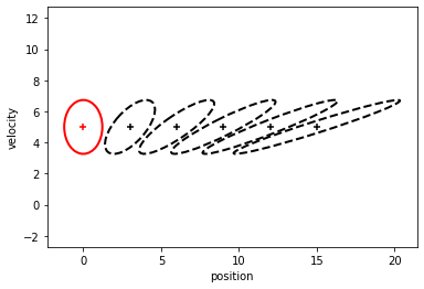
The first thing we can see is that the uncertainty on the position grows each :math:`frac{6}{10}`s.
You can notice it we the width of the ellipse.
However, the uncertainty on the velocity does not change.
Update Equations
The update equations look messier than the predict equations.
It is due to the Kalaman filter computing the update in measurement space, and measurements are not invertible.
Example
Consider a sensor that gives the range to a target. It is impossible to convert a range into a position (An infinite number of positions in a circle will yield the same range).
However, it is possible to compute the range (measurement) given a position state.
System Uncertainty
To work in measurement space the Kalman filter has to project the covariance matrix into measurement space:
where \(\bar\Sigma\) is the prior covariance and \(C\) is the measurement function.
The linear algebra is changing the coordinate system for us as in the prediction step.
With the covariance in measurement space, we add the sensor noise. Simple as they are in the same space.
The result is called the system uncertainty.
Note
Compare the equations for the system uncertainty and the covariance:
In each equation \(\Sigma\) is put into a different space with either the function \(C\) or \(A\).
Kalman Gain
If we take a look at residual diagram, we know that we need to choose a value between the prediction and the measurement.
In the univariate problem, we scaled the mean using this equation
which we simplified to
which gave us
\(K\) is the Kalman gain, and it is a real number between 0 and 1.
Ensure you understand how it selects a mean somewhere between the prediction and measurement.
The Kalman gain is a percentage or ratio - if \(K\) is .9 it takes 90% of the measurement and 10% of the prediction.
For the multivariate Kalman filter \(K\) is a vector:
Residual
The residual:
Recall that the measurement function converts a state into a measurement.
So \(C\mu\) converts \(\mu\) into an equivalent measurement.
From that, we remove the measurement \(z\) to obtain the residual.
State update
We select our new state to be along the residual, scaled by the Kalman gain:
The scaling is performed by \(Ky\), which both scale the residual and convert it back into state space with \(C^{\mathsf T}\) term which is in \(K\).
A good way to see the ratio is to rewrite the estimate equation:
The similarity between this and the univariate form should be obvious:
Covariance Update
Finally, we have the covariance update:
\(I\) is the identity matrix and \(H\) is our measurement function.
You can think of the equations as \(\Sigma = (1 -cK)\Sigma\).
\(K\) is the ratio of how much prediction vs measurement we use.
If \(K\) is large, then \((1 -cK)\Sigma\) is small and \(\Sigma\) will be made smaller than it was.
If \(K\) is small, then \((1 -cK)\Sigma\) will be relatively larger.
Meaning we adjust the size of our uncertainty by some factor of the Kalman gain.