Topic 6 - Nonlinear systems

The Kalman filter seen before consider only linear equations, meaning that you can only solve linear problems.

The world is nonlinear, so the classic Kalman filter is very limited.

Example

• Suppose we want to track an object falling through the atmosphere.

• The acceleration of the object depends on the drag it encounters.

  • Air density.

  • That decreases with altitude.

• In one dimension this can be modelled with the non-linear differential equation:

\[\ddot x = \frac{0.0034ge^{-x/22000}\dot x^2}{2\beta} - g\]

Note

Acceleration is often noted \(\ddot x\).

It’s almost true to say that the only equation that we can solve is \(Ax = B\), because we only really know how to do linear algebra.

So how, do we solve nonlinear problems?

We find a way to linearize the problem, by turning it into a set of linear equations, then we can compute an approximate solution.

How does nonlinearity create problems?

If you remember the mathematic of the Kalman filter is elegant due to the Gaussian equation being so special.

Gaussian are nonlinear, but if we add or multiply them together we still have a Gaussian!

It is something very rare, for example \(\sin x \times \sin y\) does not return a \(\sin\).

Reminder

A function to be linear has two requirements:

• additivity: \(f(x+y) = f(x) + f(y)\)

• homogeneity: \(f(ax) = af(x)\)

To illustrate this:

• Consider an audio amp.

• If I sing into a microphone, and you start talking, the output should be the sum of our voices (input) scaled by the amplifier gain.

• But if the amplifier outputs a nonzero signal such as hum for a zero input the additive relationship no longer holds.

• This is because linearity requires that \(amp(voice) = amp(voice + 0)\).

• This clearly should give the same output, but if \(amp(0)\) is nonzero, then

\[\begin{split}\begin{aligned} amp(voice) &= amp(voice + 0) \\ &= amp(voice) + amp(0) \\ &= amp(voice) + non\_zero\_value \end{aligned}\end{split}\]

• which is clearly nonsense. Hence, an apparently linear equation such as

\[L(f(t)) = f(t) + 1\]

• is not linear because \(L(0) = 1\).

Taking a look at the problem

We will consider a problem where we get the range and bearing to a target and we want to track its position.

The reported distance is 50 km, and the reported angle is \(90^\circ\).

Activity

Assume the errors in both range and angle are distributed in a Gaussian manner.

Given an infinite number of measurements what is the expected value of the position?

How does it impact Gaussians?

If you remember the Kalman filter equations (If you’re not, go there Kalman Filter Algorithm), our process function was always linear, so the output was always another Gaussian.

Now, we take an arbitrary Gaussian and we want to pass it through the function \(f(x)=5x+10\).

We could plot it directly, but let’s assume we want to sample lots of points, like 500 000 points, and use the function on them.

from numpy.random import normal

data = normal(loc=0., scale=1., size=500000)
plt.hist(5*data + 10, 1000)

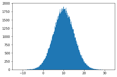
We’re not very surprise, we have a new Gaussian centered around 10.

Let us take a different look it.

def g1(x):
    return 5*x+10

plot_nonlinear_func(data, g1)

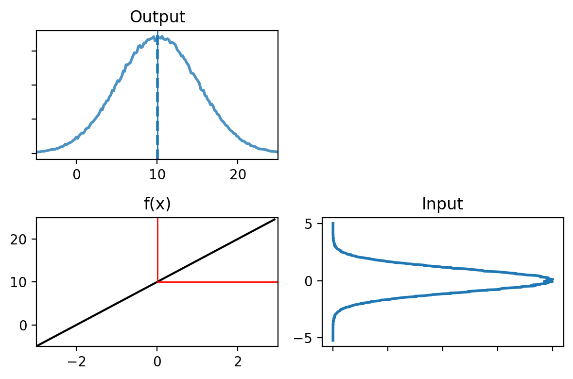
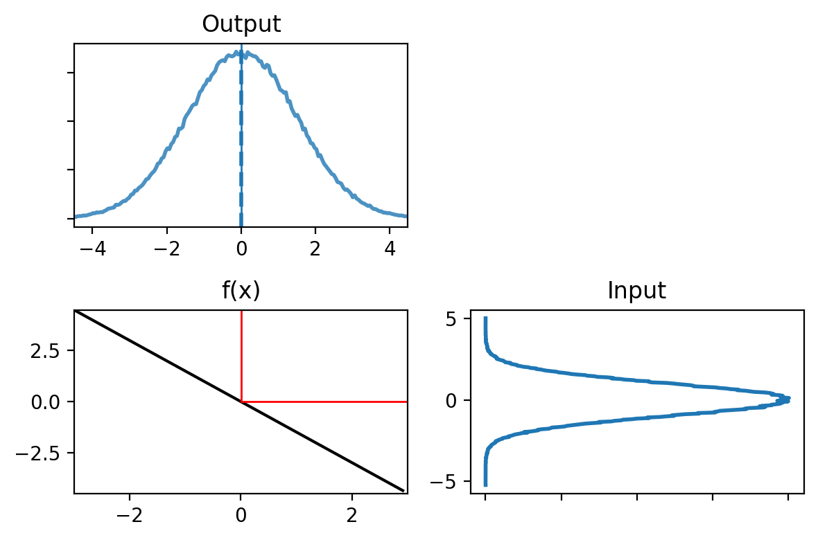
• The image labelled input are the representation of the original input data.

• The function we used is represented, and the red lines shows how \(x = 0\) is passed through the function.

• The output shows the data after being passed inside \(f(x)\).

  • The mean (the average of all the points) is represented with the dotted blue line.

  • The solid blue line shows the actual mean for the point \(x=0\).

• It looks like a Gaussian, because it is one. The \(5x\) affected the variance and the \(+10\) shifted the mean.

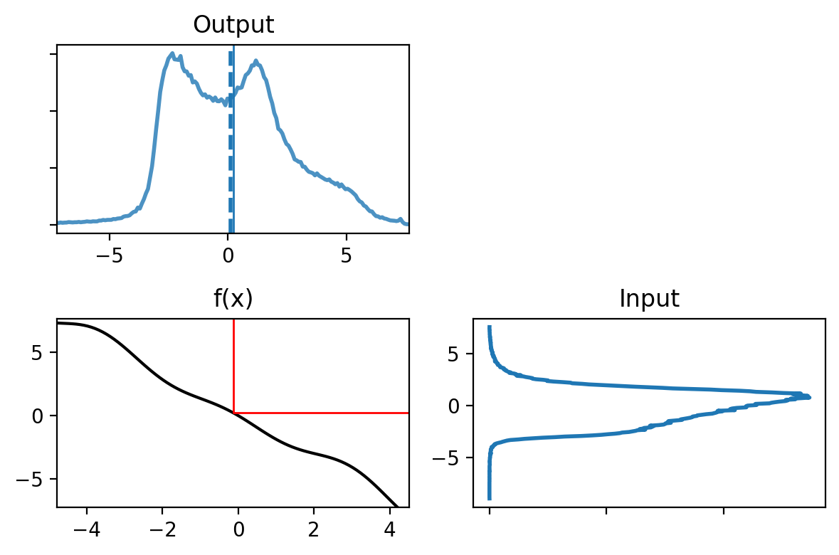
Now let’s look at a nonlinear function and see how it affects the probability distribution.

def g2(x):
    return (np.cos(3*(x/2 + 0.7))) * np.sin(0.3*x) - 1.6*x

plot_nonlinear_func(data, g2)

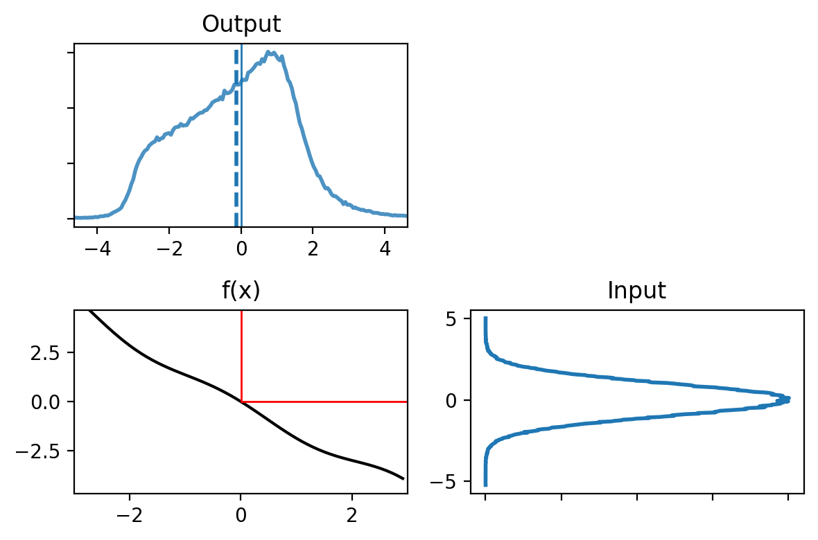
The function looks “fairly” linear, but the probability distribution of the output is completely different from a Gaussian.

Recall the equations for multiplying two univariate Gaussians:

\[\begin{split}\begin{aligned} \mu &=\frac{\sigma_1^2 \mu_2 + \sigma_2^2 \mu_1} {\sigma_1^2 + \sigma_2^2} \\ \sigma &= \frac{1}{\frac{1}{\sigma_1^2} + \frac{1}{\sigma_2^2}} \end{aligned}\end{split}\]

These equations do not hold for non-Gaussians, and certainly do not hold for the probability distribution shown in the ‘Output’ chart above.

Here’s another way to look at the same data as scatter plots.

N = 30000
plt.subplot(121)
plt.scatter(data[:N], range(N), alpha=.1, s=1.5)
plt.title('Input')
plt.subplot(122)
plt.title('Output')
plt.scatter(g2(data[:N]), range(N), alpha=.1, s=1.5)

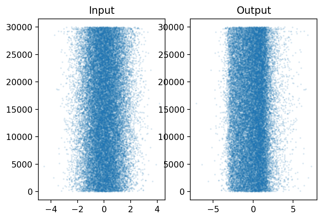
The original data seems Gaussian, while the data passed through \(g2(x)\) is no longer normally distributed.

We can see a thick band around 1.

If we pass the data through \(g2(x)\) again.

y = g2(data)
plot_nonlinear_func(y, g2)

Let’s see what the mean and variance are.

print('input  mean, variance: %.4f, %.4f' %
  (np.mean(data), np.var(data)))
print('output mean, variance: %.4f, %.4f' %
    (np.mean(y), np.var(y)))

input  mean, variance: -0.0006, 1.0033
output mean, variance: -0.1243, 2.4105

Let’s compare that to the linear function that passes through (-2,3) and (2,-3), which is very close to the nonlinear function we have plotted. Using the equation of a line we have

\[m=\frac{-3-3}{2-(-2)}=-1.5\]

def g3(x):
    return -1.5 * x

plot_nonlinear_func(data, g3)
out = g3(data)
print('output mean, variance: %.4f, %.4f' % (np.mean(out), np.var(out)))

output mean, variance: -0.0046, 2.2420

Although the shapes of the output are very different, the mean and variance of each are almost the same. This may lead you to reason that perhaps we can ignore this problem if the nonlinear equation is ‘close to’ linear. To test that, we can iterate several times and then compare the results.

out = g3(data)
out2 = g2(data)

for i in range(10):
    out = g3(out)
    out2 = g2(out2)
print('linear    output mean, variance: %.4f, %.4f' %
    (np.average(out), np.std(out)**2))
print('nonlinear output mean, variance: %.4f, %.4f' %
    (np.average(out2), np.std(out2)**2))

linear    output mean, variance: -0.2661, 7455.1775
nonlinear output mean, variance: -9.7109, 30404.1698

As you can see, it’s not true.

We have a very significant drift, and it was with a function that was very close.

Activity

Try with the function \(y(x) = -x^2\)

The code to plot is provided below:

+ show/hide code

def plot_nonlinear_func(data, f, out_lim=None, num_bins=300):
    ys = f(data)
    x0 = np.mean(data)
    in_std = np.std(data)

    y = f(x0)
    std = np.std(ys)

    in_lims = [x0 - in_std*3, x0 + in_std*3]
    if out_lim is None:
        out_lim = [y - std*3, y + std*3]

    # plot output
    h = np.histogram(ys, num_bins, density=False)
    plt.subplot(221)
    plt.plot(h[1][1:], h[0], lw=2, alpha=0.8)
    if out_lim is not None:
        plt.xlim(out_lim[0], out_lim[1])

    plt.gca().yaxis.set_ticklabels([])
    plt.title('Output')

    plt.axvline(np.mean(ys), ls='--', lw=2)
    plt.axvline(f(x0), lw=1)


    norm = stats.norm(y, in_std)

    # plot transfer function
    plt.subplot(2, 2, 3)
    x = np.arange(in_lims[0], in_lims[1], 0.1)
    y = f(x)
    plt.plot (x, y, 'k')
    isct = f(x0)
    plt.plot([x0, x0, in_lims[1]], [out_lim[1], isct, isct], color='r', lw=1)
    plt.xlim(in_lims)
    plt.ylim(out_lim)
    #plt.axis('equal')
    plt.title('f(x)')

    # plot input
    h = np.histogram(data, num_bins, density=True)

    plt.subplot(2,2,4)
    plt.plot(h[0], h[1][1:], lw=2)
    #plt.ylim(in_lims)
    plt.gca().xaxis.set_ticklabels([])
    plt.title('Input')
    plt.tight_layout()
    plt.show()

A 2D example

To illustrate even more what happen with a filter, we ca take the example of tracking an aircraft with a radar.

We first estimate the position of the aircraft.

We can try to linearize the problem.

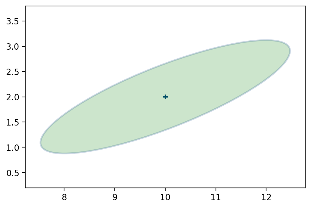
The radar is in position \(x=10\) and it gives us a range to the aircraft. The measurement is 3 km away (\(y=3\)).

The position that could match that measurement form a circle with radius 3 km:

We can see that the probable position of the aircraft is around \(x=11.4\, y=2.7\).

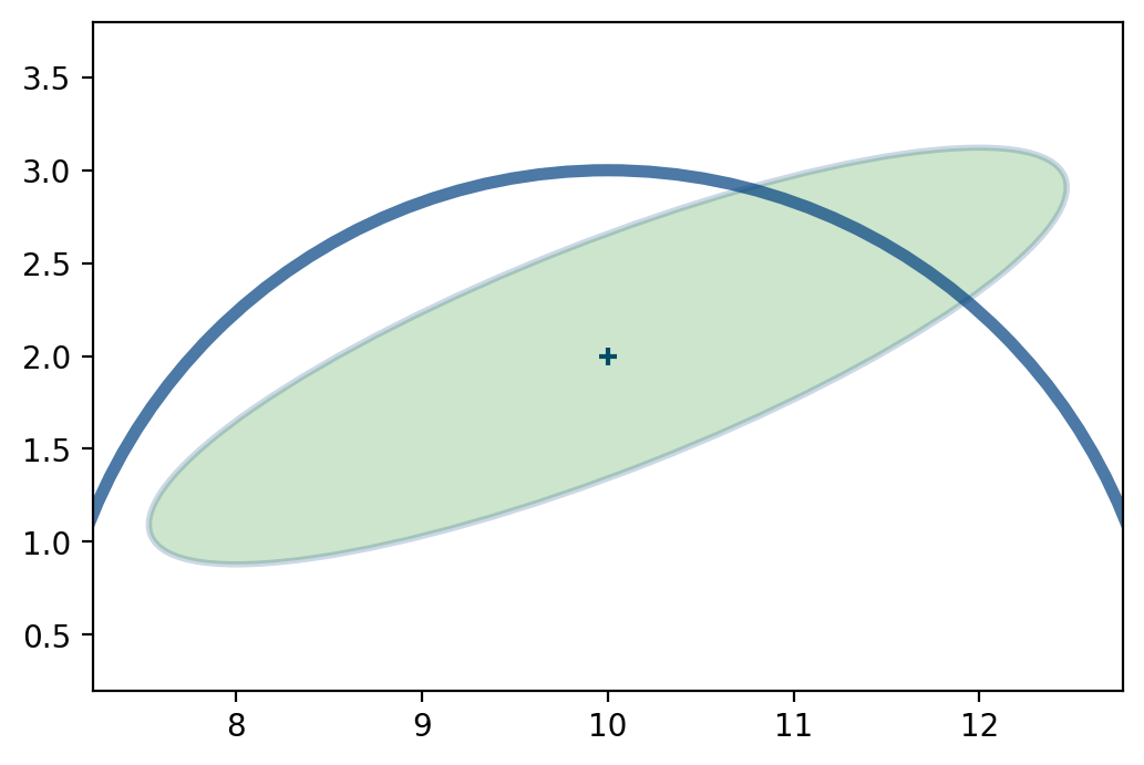
But the range measurement is non-linear, so we have to linearize it.

We haven’t covered this material yet, but the Extended Kalman filter will linearize at the last position of the aircraft (10,2). At \(x=10\) the range measurement has \(y=3\), and so we linearize at that point.

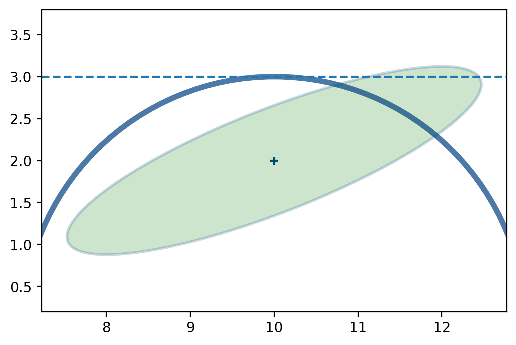
Now we have a linear function (a stright line in this case) that can be solved.

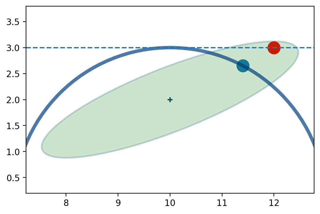
That sort of error often leads to disastrous results. The error in this estimate is large.

But in the next innovation of the filter that very bad estimate will be used to linearize the next radar measurement, so the next estimate is likely to be markedly worse than this one.

After only a few iterations the Kalman filter will diverge, and start producing results that have no correspondence to reality.