Topic 8 - Robot Motion

We have seen the filters allowing a robot to locate itself.

But we didn’t see the motion model and the measurement model of a robot.

We will focus on the motion models in this topic.

We will start with a simple definition:

Motion models

Motion models comprise the state transition probability \(p(x_t | u_t, x_{t-1})\), which plays an essential role in the prediction step.

Robot Kinematics

We need to discuss the kinematic of the robots first.

What is kinematics?

Kinematics is the calculus describing the effect of control actions on the configuration of the robot.

Usually, the configuration of a robot is commonly described by six variables:

• Its coordinates in a 3D Cartesian environment.

• 3 Eulers angles (roll, pitch and yaw) relative to an external coordinate frame.

Note

Consider that everything seen in this course is only for mobile robots.

The pose of a robot operating in a plane is represented in the figure below.

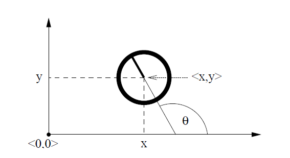
You can see the two coordinates (\(x, y\)) plus the angular orientation \(\theta\).

usually we represent it with a vector:

\[\begin{split}\begin{bmatrix} x\\ y\\ \theta\\ \end{bmatrix}\end{split}\]

be careful to not confuse it with the robot location that only contains the coordinate:

\[\begin{split}\begin{bmatrix} x\\ y\\ \end{bmatrix}\end{split}\]

The orientation of the robot is often called bearing or heading direction.

When \(\theta = 0\) the orientation of the robot is in direction of \(x\)-axis.

Probabilistic Kinematics

The motion model (or probabilistic kinematic model) is the state transition model.

It is the conditional density \(p(x_t | u_t, x_{t-1})\), where \(x_t\) and \(x_{t-1}\) are both robot poses and \(u_t\) is a motion command.

Warning

Do not mistake \(x_t\) with the \(x\) coordinate of the state!

The model describes the posterior distribution over kinematic states when a robot in state \(x_{t-1}\) executes \(u_t\).

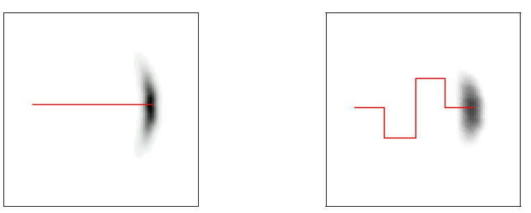
If you need to visualize it, the following figure show two robots starting in the same state \(x_{t-1}\), but executing different \(u_t\).

The shaded areas represent the likely state \(x_t\).

There are two probabilistic motion models \(p(x_t|u_t, x_{t-1})\) that can be used:

• The first assume that \(u_t\) specify the velocity command.

• The second assumes it has access to the odometry information (distance travelled, angle turned, etc.).

In practice odometry models are more accurate than velocity models.

However, odometry is only available after executing a motion command. It is logical, as you can know how far you moved after you have moved.

So, you cannot use odometry model for motion planning.

Thus odometry models are usually applied for estimation, whereas velocity models are used for probabilistic motion planning.

Velocity Motion Model

We will start with the velocity motion model.

We assume that we can control the robot by specifying two velocities:

• The rotational velocity denoted \(\omega_t\) at time \(t\).

• The translational velocity denoted \(v_t\) at time \(t\).

hence, we have:

\[\begin{split}u_t = \begin{bmatrix} v_t\\ \omega_t \end{bmatrix}\end{split}\]

Important

We will agree on a simple convention. If \(v_t > 0\) the robot has forward motion, and if \(\omega_t > 0\) it induces a counterclockwise rotation (left turns).

Closed Form Calculation

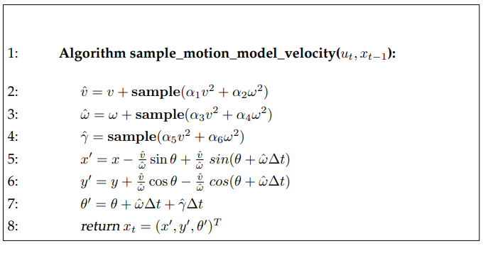
We can use the algorithm described below to calculate \(p(x_t | u_t, x_{t-1})\).

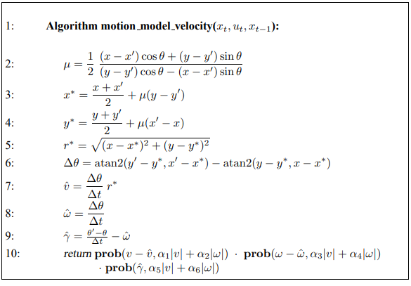
The arguments are:

• The initial pose: \(x_{t-1} = \begin{bmatrix}x & y & \theta\end{bmatrix}^T\)

• A control \(u_{t} = \begin{bmatrix}v & \omega \end{bmatrix}^T\)

• A possible successor \(x_{t} = \begin{bmatrix}x' & y' & \theta'\end{bmatrix}^T\)

It will output the probability \(p(x_t | u_t, x_{t-1})\) of being at \(x_t\) after executing \(u_t\) in \(x_{t-1}\).

The algorithm start by calculating the control of an error-free robot, then it applies the error using the function prob(a, \(b^2\)).

This function applies the motion error, by computing the probability of its parameter \(a\) under a zero-centered random variable with variance \(b^2\).

Note

The parameters \(\alpha_1, \dots, \alpha_6\) are robot-specific motion error.

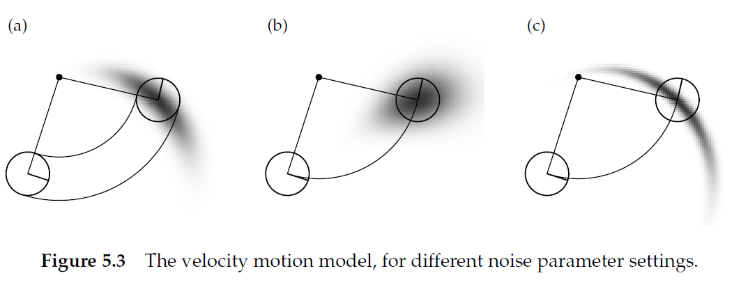
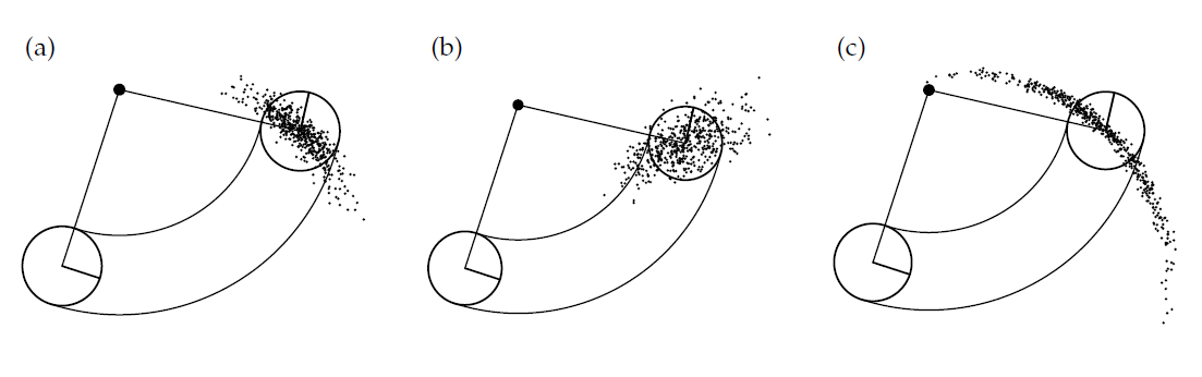
The following figure illustrates the impact of the error parameter on the estimation.

• Figure a, represent moderate errors for \(\alpha_1\) and \(\alpha_6\).

• Figure b, represent smaller angular errors for \(\alpha_3\) and \(\alpha_4\), but larger translational errors \(\alpha_1\) and \(\alpha_2\).

• Figure c, represent large angular errors, but small translational errors.

Activity

• Try to explain how the figure is coherent with the errors applied.

The prob function can be applied in two different ways, as described below.

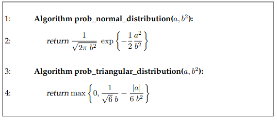
Note

The rand(x, y) function is assumed to be a pseudo-random number generator with uniform distribution(in \([x, y]\)).

Sampling Algorithm

It is sometimes, easier to sample from a conditional density than calculating the density.

Indeed, when you’re sampling you use \(u_t\) and \(x_{t-1}\) and seeks to generate a random \(x_t\) using \(p(x_t| u_t, x_{t-1})\).

In contrary to calculating the density, in which you need to give \(x_t\) that you will generate with other means to calculate \(p(x_t| u_t, x_{t-1})\).

The algorithm is described below:

The arguments are:

• The initial pose: \(x_{t-1} = \begin{bmatrix}x & y & \theta\end{bmatrix}^T\)

• A control \(u_{t} = \begin{bmatrix}v & \omega \end{bmatrix}^T\)

We still find the 6 parameters representing the motion error.

To sample the different values we can use the following algorithms:

Note

The rand(x, y) function is assumed to be a pseudo-random number generator with uniform distribution(in \([x, y]\)).

Now if we use the same example and sample 500 samples, we obtain the following figure.

As you can see the shape of the samples is very similar to the density function calculated with the previous algorithm.

Activity

1. Implement the sample_normal_distribution function in python.

2. Implement the sample_motion_model_velocity(u, x, dt, alpha, sample) function in python.

   • u being the control vector

   • x being the state \(x_{t-1}\)

   • dt being \(\Delta t\)

   • alpha the vector containing all the errors \(\alpha_1, \dots, \alpha_6\).

   • sample the sampling function you want to use.

3. Test the motion model velocity function for different values.

Odometry Motion Model

The velocity motion model we have seen before uses the robot’s velocity to compute posterior over poses.

Instead of velocity motion, it is possible to use the odometry measurement to estimate the robot’s motion over time.

Note

In practice odometry is usually more accurate than velocity.

However, the odometry is only available in retrospect, after the robot moved.

It is not an issue for the filter algorithm or localization and mapping algorithms, but it cannot be used for accurate motion planning.

Closed Form Calculation

Odometry is working very differently from velocity, because technically odometric information are sensor measurements, not controls.

First, we will see the format of our control information.

At time \(t\), the correct pose of the robot is modelled by the random variable \(x_t\).

The robot odometry estimate this pose, but due to drift and slippage there is no fixed coordinate transformation between the robot’s internal odometry and the physical world coordinates.

Why???

The odometry model uses relative motion information. You have information such as the robot move 2m forward, which is relative to the previous state, and it contains errors.

More specifically, in the time interval \((t-1, t]\), the robot advances from a pose \(x_{t-1}\) to pose \(x_t\). But the odometry reports back to us a related advance from \(\bar{x}_{t-1} = [\bar x \quad \bar y \quad \bar \theta]^T\) to \(\bar{x}_{t} = [\bar x' \quad \bar y' \quad \bar \theta']^T\).

The bar indicates that these are odometry measurements embedded in a robot internal coordinate whose relation to the global world coordinates is unknown.

The motion information \(u_t\) is given by the pair:

\[\begin{split}u_t = \begin{bmatrix} \bar{x}_{t-1}\\ \bar{x}_{t} \end{bmatrix}\end{split}\]

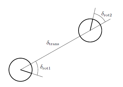
So to transform it to a control/motion information we calculate the relative difference in three steps:

• A rotation, denoted \(\delta_{rot1}\)

• A translation, straight line motion, denoted \(\delta_{trans}\)

• A rotation, denoted \(\delta_{rot2}\)

The following figure illustrates the three steps.

Activity

• Convince yourself that there is a unique parameter vector \([\delta_{rot1} \quad \delta_{trans} \quad \delta_{rot2}]^T\) for each pair of position \((\bar x, \bar x')\).

• It is sufficient to reconstruct the relative motion between \(\bar x\) and \(\bar x'\).

Of course the probabilistic motion model assumes that these three parameters are corrupted by independent noise.

Note

There is one more parameter in the odometry motion than in the velocity vector.

Now we can finally take a look at the algorithm.

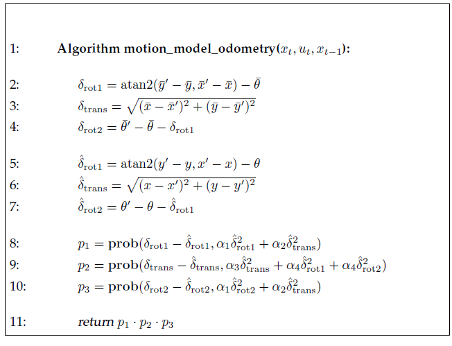
The arguments are:

• The initial pose: \(x_{t-1} = \begin{bmatrix}x & y & \theta\end{bmatrix}^T\)

• A control \(u_{t} = \begin{bmatrix}\bar{x}_{t-1} & \bar{x}_{t} \end{bmatrix}^T\)

• A possible successor \(x_{t} = \begin{bmatrix}x' & y' & \theta'\end{bmatrix}^T\)

If we analyze the algorithm:

• Lines 2 to 4 recover relative motion parameters \([\delta_{rot1} \quad \delta_{trans} \quad \delta_{rot2}]^T\)

• Lines 5 to 7 calculates the relative motion parameters \([\hat{\delta}_{rot1} \quad \hat{\delta}_{trans} \quad \hat{\delta}_{rot2}]^T\)

• Lines 8 to 10 calculates the error probabilities for individual motion parameters.

Important

• All angular differences must lie in \([-\pi, \pi]\).

• Hence the outcome of \(\delta_{rot2} - \bar{\delta}_{rot2}\) must be truncated.

In this case we only have 4 error parameters, \(\alpha_1, \dots, \alpha_4\), that are also robot specific.

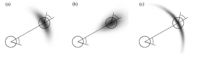
The following figure show some examples of the probability distribution for different error parameters.

• Figure a, represent a typical distribution.

• Figure b, represents an unusually large translational error.

• Figure c, represents an unusually large rotational error.

Sampling Algorithm

The idea is similar to the sample algorithm for velocity motion model.

We don’t calculate the distribution, we sample it.

The algorithms is described below:

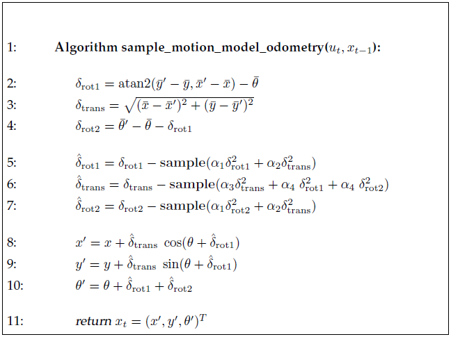
The arguments are:

• The initial pose: \(x_{t-1} = \begin{bmatrix}x & y & \theta\end{bmatrix}^T\)

• A control \(u_{t} = \begin{bmatrix}\bar{x}_{t-1} & \bar{x}_{t} \end{bmatrix}^T\)

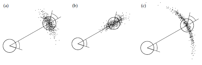
The following figure shows examples of samples generated with the algorithm following the same type of errors from the previous example.

Activity

1. Implement the sample_motion_model_velocity(u, x, dt, alpha, sample) function in python.

   • u being the vector \(u_{t} = \begin{bmatrix}\bar{x}_{t-1} & \bar{x}_{t} \end{bmatrix}^T\)

   • x being the state \(x_{t-1}\)

   • alpha the vector containing all the errors \(\alpha_1, \dots, \alpha_4\).

   • sample the sampling function you want to use.

2. Test the motion model odometry function for different values.