Topic 2 - Probabilities
Why are we talking about probabilities?
Working with mobile robots, it’s working with uncertainty.
Uncertainty can come from the error in the motion control.
Uncertainty can come from the measurement errors of the sensors.
To reduce the uncertainty, we need an explicit representation of the uncertainty.
The uncertainty is often represented with probability theory.
Probabilistic inference is the process of calculating these laws for random variables that are derived from other random variables and the observed data.
Discrete Random Variables
Important
This is something that you should already know!
We denote \(X\) a random variable.
And \(x\) a value that X could take.
\(p(X=x)\) or \(p(x)\) represents the probability that \(X\) takes the value \(x\).
Example
If you flip a coin that you can obtain ever heads or tails.
\(p(X=head)=p(X=tail)=\frac{1}{2}\)
Discrete probabilities always sum to 1:
Note
Probabilities are always non-negative: \(p(X=x)\ge 0\).
Continuous Random Variables
You will see that in robotics, we usually address estimation and decision-making in continuous spaces.
We denote \(X\) is a random continuous variable.
We assume that all continuous random variable possesses probability density functions (PDFs).
Activity
Can you give me one common density function?
A very common one:
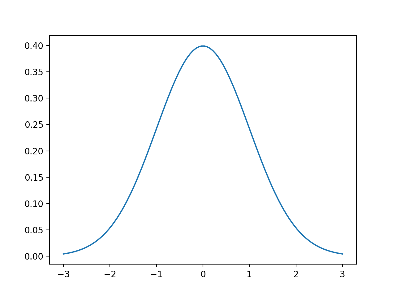
The one-dimensional normal distribution with mean \(\mu\) and variance \(\sigma^2\).
The PDF of a normal distribution is a Gaussian function.
- Gaussian function
PDF: \(p(x)=(2\pi\sigma^2)^{-\frac{1}{2}}\exp\{-\frac{1}{2}\frac{(x-\mu)^2}{\sigma^2}\}\)
Abbreviation: \(\mathcal{N}(x;\mu;\sigma^2)\)
\(x\) is a scalar value.
Example
import matplotlib.pyplot as plt
import numpy as np
import scipy.stats as stats
import math

mu = 0
variance = 1
sigma = math.sqrt(variance)
x = np.linspace(mu - 3*sigma, mu + 3*sigma, 100)
plt.plot(x, stats.norm.pdf(x, mu, sigma))
plt.show()
If we have more than one parameter:
\(x\) becomes a multi-dimensional vector.
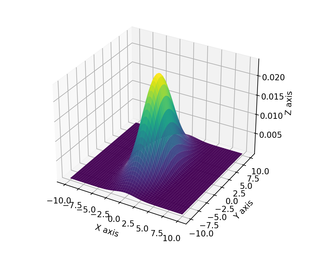
Normal distributions over vectors are called multivariate
- Multivariate normal distribution
PDF: \(p(x)=\det (2\pi\Sigma)^{-\frac{1}{2}}\exp\{-\frac{1}{2}(x-\mu)^T\Sigma^{-1}(x-\mu)\}\)
covariance matrix: \(\Sigma\) is a positive semidefinite and symmetric matrix.
As discrete probabilities, continuous probabilities always sums to 1:
Example
import numpy as np
import matplotlib.pyplot as plt
from scipy.stats import multivariate_normal
from mpl_toolkits.mplot3d import Axes3D

#Parameters to set
mu_x = 0
variance_x = 3

mu_y = 0
variance_y = 15

#Create grid and multivariate normal
x = np.linspace(-10,10,500)
y = np.linspace(-10,10,500)
X, Y = np.meshgrid(x,y)
pos = np.empty(X.shape + (2,))
pos[:, :, 0] = X; pos[:, :, 1] = Y
rv = multivariate_normal([mu_x, mu_y], [[variance_x, 0], [0, variance_y]])

#Make a 3D plot
fig = plt.figure()
ax = fig.gca(projection='3d')
ax.plot_surface(X, Y, rv.pdf(pos),cmap='viridis',linewidth=0)
ax.set_xlabel('X axis')
ax.set_ylabel('Y axis')
ax.set_zlabel('Z axis')
plt.show()
Joint and Conditional probability
- Joint distribution
Formula: \(p(X=x \text{ and } Y=y) = p(x,y)\)
- Independence
Formula: \(p(x)p(y) = p(x,y)\)
Definition: Describes the probability of the event that the random variable \(X\) takes on the value \(x\) and that \(Y\) takes on the value \(y\).
- Conditional probability
Formula: \(p(X=x|Y=y) = p(x|y)\)
Definition: Knowing \(y\), the probability that \(X=x\) is conditioned to \(y\).
If \(p(y)>0\) then the conditional probability is defined as:
\[p(x|y) = \frac{p(x,y)}{p(y)}\]If \(Y\) and \(X\) are independent:
\[p(x|y) = \frac{p(x)p(y)}{p(y)} = p(x)\]
Law of Total Probability, Marginals
From the definition of the conditional probability and the axioms of probability measures is referred to as Theorem of total probability.
In the discrete case: \(p(x)=\sum_y p(x|y)p(y)\).
In the continuous case: \(p(x) = \int p(x|y)p(y)dy\).
Bayes formulas
- Bayes rule
Discrete case:
\[p(x|y) = \frac{p(y|x)p(x)}{p(y)} = \frac{p(y|x)p(x)}{\sum_{x'}p(y|x')p(x')}\]Continuous case:
\[p(x|y) = \frac{p(y|x)p(x)}{p(y)} = \frac{p(y|x)p(x)}{\int p(y|x')p(x')dx'}\]
Why is this important?
If \(x\) is a quantity that we would like to infer from \(y\) (like a position).
The probability \(p(x)\) will be referred as the prior probability distribution and \(y\) is called the data (sensor measurement).
\(p(x)\) summarize the knowledge we have on \(X\) prior to incorporating the data \(y\).
\(p(x|y)\) is called the posterior probability distribution over \(X\).
The Bayes formula can be formulated as:
Note
\(p(y)\) does not depend on \(x\). Thus \(p(y)^{-1}\) is the called the normalizer and denoted \(\eta\).
\(p(x|y) = \eta p(y|x)p(x)\)
Activity
You are planning a picnic today, but the morning is cloudy.
Oh no! 50% of all rainy days start off cloudy!
But cloudy mornings are common (about 40% of days start cloudy)
And this is usually a dry month (only 3 of 30 days tend to be rainy, or 10%)
What is the chance of rain during the day?
We will use Rain to mean rain during the day, and Cloud to mean cloudy morning.
The chance of Rain given Cloud is written P(Rain|Cloud).
Conditioning
We can condition the Bayes rule on more than one variable.
For example, we can have a condition on \(Z = z\):
as long as \(p(y|z)>0\).
It also means that \(p(x|y)=\int p(x|y,z)p(z|y)dz\).
Similarly, we can condition the rule for combining probabilities of independent random variables on other variables \(z\):
Such a relation is known as conditional independence. And it is equivalent to
\(p(x|z) = p(x|z,y)\)
\(p(y|z) = p(y|z,x)\)
Expectations of random variables
The expected value of random variable is denoted \(E[X]\).
You can think of it as the “average” value attained by random variable.
In fact, it also called its mean.
- Expected value
discrete case: \(E[X] = \sum_x xp(X=x)\)
continuous case: \(E[X]=\int xp(x)dx\)
Activity
Calculate the expected value of a roll of die.
- Covariance
The covariance measure the squared expected deviation from the mean.
\(\text{Cov}[X] = E[X-E[X]]^2 =E[X^2]-E[X]^2\)