Topic 10 - Markov Decision Process
Until now we have seen how a robot move or locate itself.
It is important now to cover how a robot can plan its mission.
We will now cover probabilistic algorithms.
Motivation
We can take a few examples:
A robotic manipulator grasp and assembles parts arriving in random configuration on a conveyor belt.
The parts that arrive are unknown.
The optimal strategy requires to know the future parts.
A vehicle to move from point A to point B in Toronto.
Shall it take the shortest path through downtown, but losing the GPS.
Or shall it takes the longest path, but keeping the GPS.
Robots need to map an area collectively.
Should they seek each other?
Or should they cover more unknown area alone?
In robotics we need to consider two types of uncertainties:
Uncertainty of the actions.
Uncertainty on the measurement.
Activity
How would you handle these two uncertainties?
Markov Decision Process
We will star by tackling the problem of the uncertainty on the actions.
Markov Decision Process or called MDP is a mathematical framework that allows us to consider stochastic environment.
The Idea
MDPs can be represented graphically as follows:
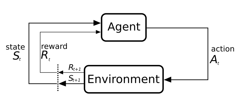
We have an agent, in our case a robot.
These agents evolve in an environment.
The agent can interact with this environment with different actions.
When the agent uses an action it changes the state of the environment and it gives it a reward.
Activity
Consider a robot that needs to navigate in a maze.
Try to answer the following questions:
What would be the environment?
What would be the actions?
What would be the state?
Formally
We need to define MDPs formally.
Definition
A MDP is defined with a tuple \((S,A,T,R)\):
\(S\) is the state space that contains the set of states \(s\in S\).
\(A\) is the action space that contains the set of actions \(a\in A\).
\(T: S\times A\times S\) is the transition function that defines the probability \(p(s_{t+1}=s'|s_{t}=s,a_{t})\).
\(R: S\times A \rightarrow \mathbb{R}\) is the reward function that defines \(r(s,a)\).
Activity
Remember the problem of detecting Alan in the hallway?
Alan can only move forward.
At each time step, Alan can ever overshoot by 1 cell with a probability of 10%.
Alan can ever undershoot by 1 cell with a probability of 10%.
Now we want to model Alan moving in the hallway as an MDP:
Define the state space.
Define the action space.
Define the transition function.
Solving a MDP
The strategy in an MDP is called a policy \(\pi: S \rightarrow A\).
It’s a function that gives for each state \(s\in S\) the action \(a\in A\).
When a policy is followed we obtain a trajectory \(G\).
Which is a sequence of rewards:
where \(\gamma\) is a discount rate \(0 \leq \gamma \leq 1\).
The discount rate determines the present value of future rewards.
When the discount rate approaches 1, the future rewards are taken into account more strongly.
The objective of the MDPs is to calculate the optimal policy \(\pi^*\).
The policy that will maximize the value function \(V^\pi(s_0)\).
\(V^\pi(s_0)\) is the total expected reward if the agent follow \(\pi\) starting in \(s_0\):
So the optimal value function \(V^{\pi^*}\) is defined as:
Dynamic Programming
We define how a MDP can be solved, but we need to discuss possible algorithms to do it.
MDPs are usually solved dynamic programming algorithms.
We will assume a finite MDP (finite horizon).
The Idea
We want to use the value functions to search for a good policy.
We have seen that we can obtain the optimal policy once we found the optimal value function.
The idea is to calculate the optimal value function.
Value Iteration
Value Iteration is an exact method.
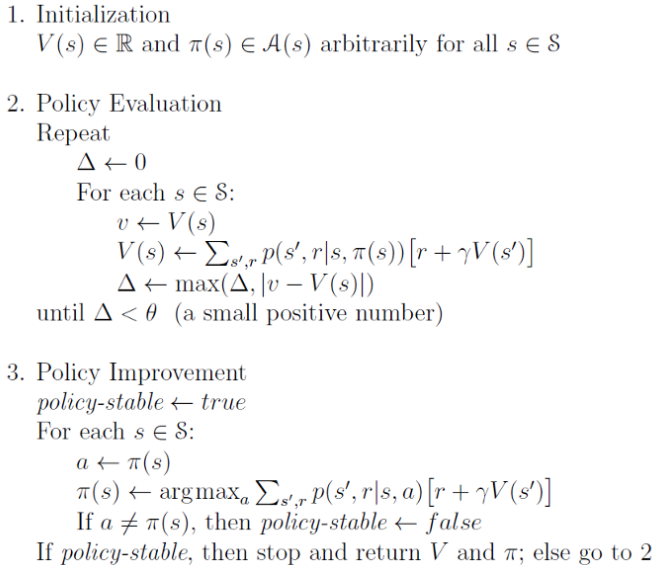
It works in three steps:
Initialize random policy
Policy Evaluation
Policy improvement
Pseudocode
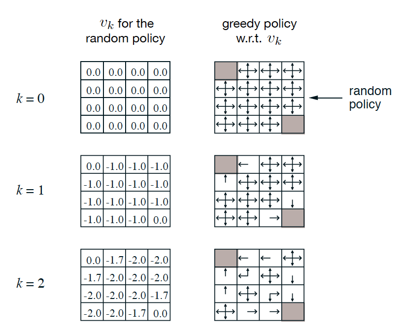
Example
A robot that needs to either go on the cell on the top left or bottom right cell.
At first the policy is initialized randomly.
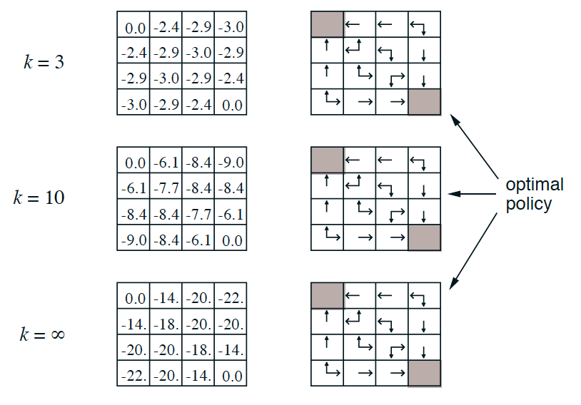
After applying policy iteration we converge to the optimal policy.
Activity
Consider the following problems:
A Hallway consisting of 7 tiles.
The idea is for a robot to reach the centered tile.
It can start from any tile.
It can either move on the left or on the right.
Each time the robot moves it receive a reward of -1.
If it reaches the centered tile, it receives a reward of +10.
Model this as an MDP.
Solve it by hand.
Implement it in python.
Efficiency
Dynamic programming is very efficient for lots of problems.
It is also the case with Markov Decision Processes.