Topic 7 - Kalman Filters for Nonlinear Systems

We have seen the difficulties that nonlinear systems pose in the previous topic.

The nonlinearity can appear in two places:

• In the measurement model

• In the process model

As the Kalman filter performs poorly or not at all with these systems, researchers proposed to extension of the Kalman filter for nonlinear systems.

We will cover two of them:

• The Unscented Kalman Filter

• The Extended Kalman Filter

The Unscented Kalman Filter (UKF)

We have seen in the previous topic that we can have nonlinear functions.

Consider the following function:

# create 500,000 samples with mean 0, std 1
Gaussian = (0., 1.)
data = normal(loc=gaussian[0], scale=gaussian[1], size=500000)

def f(x):
    return (np.cos(4*(x/2 + 0.7))) - 1.3*x

plot_nonlinear_func(data, f)

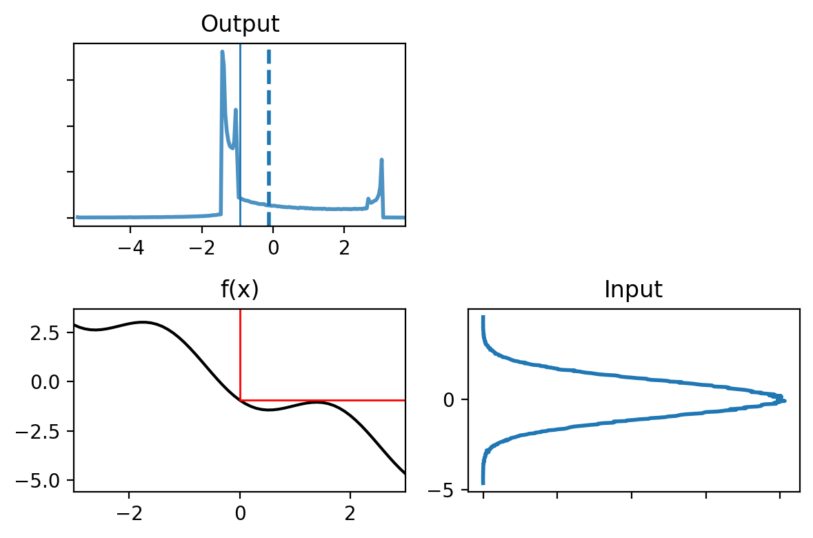
We generated 500 000 samples from the input, that we passed through the nonlinear function.

If we take a look at the scatter plot:

N = 30000
plt.subplot(121)
plt.scatter(data[:N], range(N), alpha=.2, s=1)
plt.title('Input')
plt.subplot(122)
plt.title('Output')
plt.scatter(f(data[:N]), range(N), alpha=.2, s=1)

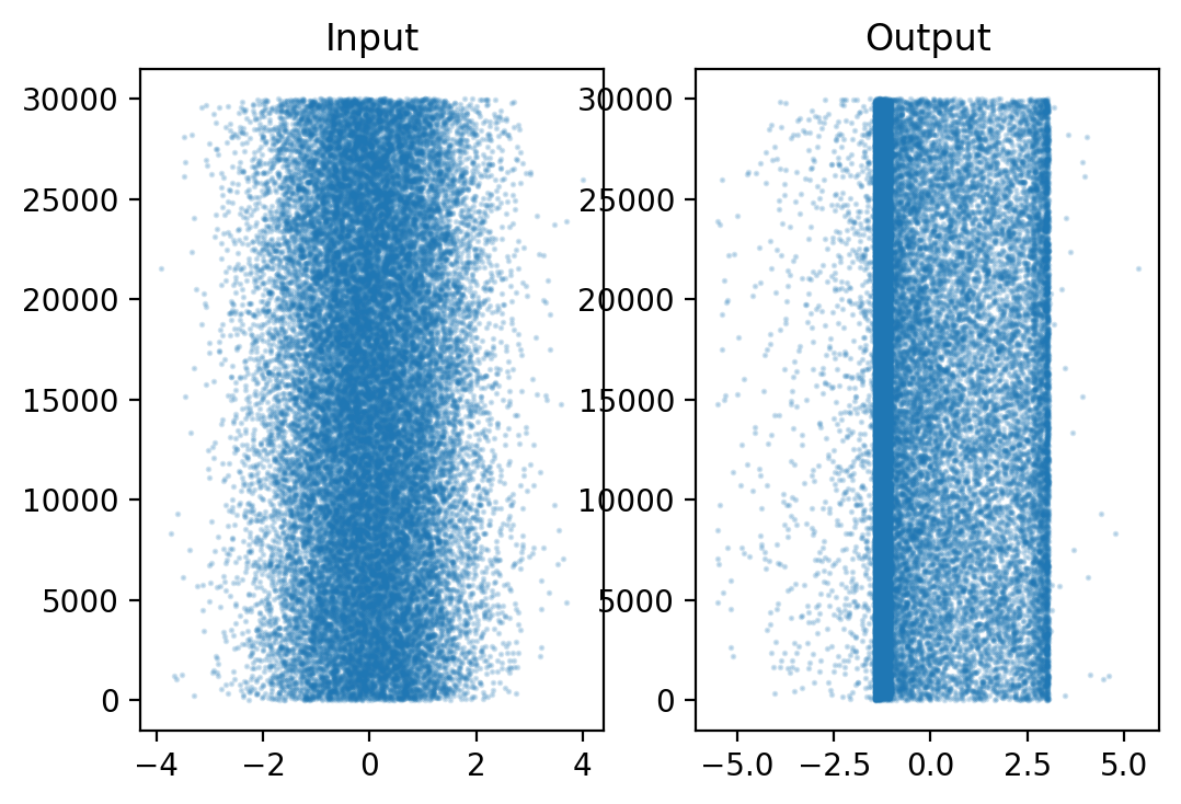
We can see that the data is no longer Gaussian. We can distinguish two bands with a significant number of points in between.

Having a lot of points can be very interesting. If we update the mean and variance with the sample points, we could approximate a Gaussian.

This idea is the Monte Carlo approach.

• You generate a lot of points to have a good approximation of the real distribution.

• Gnerating points takes a lot of computational power.

• Even 500 000 points are not enough, but it is already a computational burden.

This is why the unscented Kalman filter uses sigma points to reduce the amount of computation by using a deterministic method to choose the points.

Sigma Points - Sampling from a Distribution

In this part we will consider 2D Gaussians, because they are easy to plot.

Note

It extends to any number of dimensions.

The idea:

• Assume a nonlinear function.

• We take random points from the covariance ellipse.

• Pass the points through the non linear function.

• We compute the mean and covariance of the transformed points.

• We use them as our new estimate.

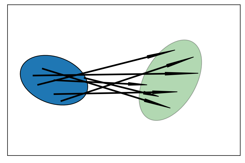
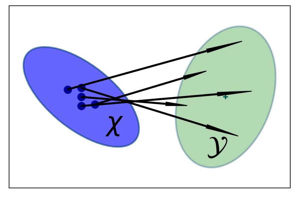
• The figure depicts the \(1\sigma\) distribution of the two state variables.

• The arrows show how several randomly sampled points might be transformed by an arbitrary function.

• The ellipse on the right is the new estimate.

Activity

• Consider the following Gaussian:

\[\begin{split}\mu = \begin{bmatrix}0\\0\end{bmatrix}, \Sigma=\begin{bmatrix}32&15\\15&40\end{bmatrix}\end{split}\]

• And the following nonlinear system:

\[\begin{split}\begin{cases}\begin{aligned}\bar x&=x+y\\ \bar y&= 0.1x^2 + y^2\end{aligned} \end{cases}\end{split}\]

• Generate randomly 10 000 points from the initial Gaussian.

• Implement the nonlinear function f_nonlinear_xy(x, y).

• Linearize the function:

mean_fx = f_nonlinear_xy(*mean)

• Use the following function plot_monte_carlo_mean(xs, ys, f_nonlinear_xy, mean_fx, 'Linearized Mean'):

Here is a code to plot the Gaussian:

+ show/hide code

from scipy import stats

def plot_bivariate_colormap(xs, ys):
    xs = np.asarray(xs)
    ys = np.asarray(ys)
    xmin = xs.min()
    xmax = xs.max()
    ymin = ys.min()
    ymax = ys.max()
    values = np.vstack([xs, ys])
    kernel = stats.gaussian_kde(values)
    X, Y = np.mgrid[xmin:xmax:100j, ymin:ymax:100j]
    positions = np.vstack([X.ravel(), Y.ravel()])

    Z = np.reshape(kernel.evaluate(positions).T, X.shape)
    plt.gca().imshow(np.rot90(Z), cmap=plt.cm.Greys,
                    extent=[xmin, xmax, ymin, ymax])

def plot_monte_carlo_mean(xs, ys, f, mean_fx, label, plot_colormap=True):
    fxs, fys = f(xs, ys)

    computed_mean_x = np.average(fxs)
    computed_mean_y = np.average(fys)

    ax = plt.subplot(121)
    ax.grid(b=False)

    plot_bivariate_colormap(xs, ys)

    plt.scatter(xs, ys, marker='.', alpha=0.02, color='k')
    ax.set_xlim(-20, 20)
    ax.set_ylim(-20, 20)

    ax = plt.subplot(122)
    ax.grid(b=False)

    plt.scatter(fxs, fys, marker='.', alpha=0.02, color='k')
    plt.scatter(mean_fx[0], mean_fx[1],
                marker='v', s=300, c='r', label=label)
    plt.scatter(computed_mean_x, computed_mean_y,
                marker='*',s=120, c='b', label='Computed Mean')

    plot_bivariate_colormap(fxs, fys)
    ax.set_xlim([-100, 100])
    ax.set_ylim([-10, 200])
    plt.legend(loc='best', scatterpoints=1)
    print ('Difference in mean x={:.3f}, y={:.3f}'.format(
        computed_mean_x-mean_fx[0], computed_mean_y-mean_fx[1]))

Choosing Sigma Points

We discussed the number of points we need to generate to obtain a good estimation.

We used 500 000 points at the beginning of the topic to estimate a new Gaussian, but choosing 500 000 points for every update would cause our filter to be extremely slow.

So, how many points do we need?

If we consider the simplest possible case, it is the indentity function \(f(x)=x\).

• If our filter does not work for the identity function then the filter cannot converge.

• If the input is 1, the output must also be 1.

• If the output was different such as 1.1, then we will feed 1.1.

• We could get another number again 1.23.

• Meaning it will diverge.

One point

The fewest number of points that we can use is one per dimension. This is the number of the linear Kalman filter uses.

The input to a Kalman filter for the distribution \(\mathcal{N}(\mu,\sigma^2)\) is \(\mu\) itself. So while this works for the linear case, it is not a good answer to the nonlinear case.

We could use one altered point per dimension, but if we were to pass some value \(\mu + \Delta\) into the identity function, it would not converge either.

So we need more points.

Two points

The next lower number is two and considering that Gaussians are symmetric, and that we probably want to always have one of our sample points is the mean of the input for the identity function to work.

Two points would require us to select the mean, and then one other point.

It would introduce an asymmetry in our input that we don’t really want.

Three points

The next lower number of points is 3.

We could have the mean and two points to keep the symmetry.

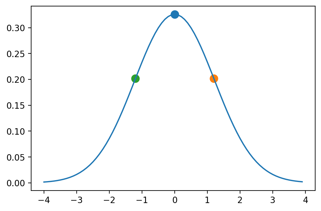
If we take these points through a nonlinear function \(f(x)\) and compute the resulting mean and variance.

Calculating mean with 3 points is not very general.

For example, for a very nonlinear problem we might want to weight the center point much higher than the outside points, or we might want to weight the outside points higher.

General approach

We want to compute the weighted mean:

\[\mu = \sum_i w^i f(\mathcal X)\]

where \(\mathcal X\) are the sigma points.

Of course the sums of the weights must be equal to one, so it is important to select \(\mathcal X\) and their corresponding weights.

If we weight the means, we need to weight the covariances. It is possible to use different weights for the mean (\(w_m\)) and for the covariance (\(w_c\)).

We obtain our constraints:

\[\begin{split}\begin{aligned} 1 &= \sum_i w_m^i\\ 1 &= \sum_i w_c^i\\ \mu &= \sum_i w_m^i f(\mathcal X)\\ \Sigma &= \sum_i w_c^i(f(\mathcal X)^i-\mu)(f(\mathcal X)^i-\mu)^T) \end{aligned}\end{split}\]

The calculation of the covariance may be less familiar, but remember the equation for the covariance of two random variables:

\[COV(x,y) = \frac{\sum(x-\bar x)(y-\bar y)}{n}\]

Note

These constraints do not form a unique solution, we use different weights between for the mean and covariances.

The only thing that is very important to understand is that there are infinite ways to select sigma points.

The Unscented Transform

For now, we will consider that we can select sigma points and calculate their weights.

We will see how we can use these points to implement a filter.

The unscented transform is simple, but it is the core of the algorithm. It passes the sigma points \(\mathcal X\) through a nonlinear function yielding a transformed set of points:

\[\mathcal Y = f(\mathcal X)\]

Graphically we obtain:

We can rewrite the mean and covariance equation:

\[\begin{split}\begin{aligned} \mu &= \sum_{i=0}^{2n}w_m^i\mathcal Y^i\\ \Sigma &= \sum_{i=0}^{2n} w_c^i(\mathcal Y^i-\mu)(\mathcal Y^i-\mu)^T \end{aligned}\end{split}\]

Note

The name “unscented” might be confusing. It doesn’t really mean much. It was a joke fostered by the inventor that his algorithm didn’t “stink”, and soon the name stuck. There is no mathematical meaning to the term.

If we generate sigma points with their corresponding weights and we apply the unscented transform, we obtain the following:

Activity

Implement the function unscented_transform(sigmas_f, Wm, Wc), where:

• sigmas_f are the points after nonlinear transformation

• Wm and Wc are the weights.

The function will return the mean and covariance.

Use the following value:

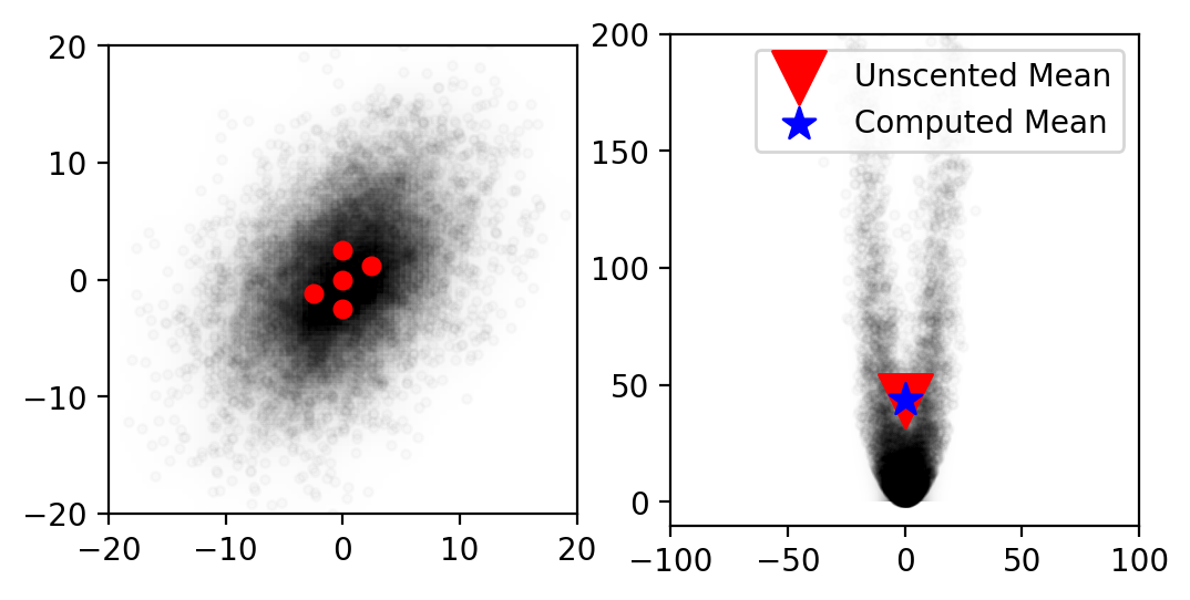
+ show/hide code

sigmas_f = [ 0.          0.        ]
           [ 3.61205015  1.93370625]
           [ 2.49621589  6.23109375]
           [-3.61205015  1.93370625]
           [-2.49621589  6.23109375]]
Wm = [-9.58201058  2.64550265  2.64550265  2.64550265  2.64550265]
Wc = [-6.67201058  2.64550265  2.64550265  2.64550265  2.64550265]

Then use the previous function plot_monte_carlo_mean to plot the new Gaussian.

As you can see, the difference is impressive. This filter is one of the most efficient ones.

The Unscented Kalman Filter

It is now possible to present the UKF.

Predict Step

The UKF’s predict step computes the prior using the process model \(f()\), \(f()\) being a nonlinear function.

We obtain \(\mathcal X\) and the weights \(w_m, w_c\):

\[\begin{split}\begin{aligned} \boldsymbol\chi &= \text{sigma-function}(\mu, \Sigma) \\ w_m, w_c &= \text{weight-function}(\mathtt{n, parameters}) \end{aligned}\end{split}\]

We pass each sigma points through \(f(\mu, \Delta t)\):

\[\mathcal Y = f(\mathcal X, \Delta t)\]

We compute the mean and covariance of the prior using the unscented transform on the transformed sigma points:

\[\begin{split}\begin{aligned} \bar \mu &=\sum_{i=0}^{2n}w_m^i\mathcal Y^i\\ \bar\Sigma &= \sum_{i=0}^{2n} w_c^i(\mathcal Y^i-\bar\mu)(\mathcal Y^i-\bar\mu)^T + R \end{aligned}\end{split}\]

If you want to compare with the Kalman filter:

\[\begin{split}\begin{array}{l|l} \text{Kalman} & \text{Unscented} \\ \hline & \mathcal Y= f(\chi) \\ \bar \mu = A\mu & \bar \mu = \sum w_m\mathcal Y \\ \bar \Sigma = APA^T + R & \bar \Sigma = \sum w_c(\mathcal Y-\bar\mu)(\mathcal Y-\bar\mu)^T + R \end{array}\end{split}\]

Update Step

Important

Remember that Kalman filter perform the update in measurement space.

We need to convert the sigma points of the prior into measurements using a measurement function \(h(x)\) that you define:

\[\mathcal Z = h(\mathcal Y)\]

Similarly to the prediction step we apply the unscented transform to these points:

\[\begin{split}\begin{aligned} \hat z &= \sum_{i=0}^{2n} w_m^i\mathcal Z^i\\ S &= \sum_{i=0}^{2n}w_c^i(\mathcal Z^i - \hat z)(\mathcal Z^i - \hat z)^T + Q\\ \end{aligned}\end{split}\]

The residual of the measurement \(z\) is trivial to compute:

\[y = z- \hat z\]

To compute the Kalman gain we first compute the cross covariance of the state and the measurements, which is defined as:

\[\begin{split}\bar\Sigma^{x,z} = \sum_{i=0}^{2n}w_c^i(\mathcal X^i - \bar\mu)(\mathcal Z^i - \hat z)^T\\\end{split}\]

And th Kalman gain is defined as:

\[K = \bar\Sigma^{x,z}S^{-1}\]

If you think of the inverse as a kind of matrix reciprocal, you can see that the Kalman gain is a simple ratio which computes:

\[K \approx \frac{\bar\Sigma^{x,z}}{S} \approx \frac{\text{belief in state}}{\text{belief in measurement}}\]

Finally, we compute the new state estimate using the residual and Kalman gain:

\[\mu = \bar\mu + Ky\]

and the new covariance is computed as:

\[\Sigma = \bar\Sigma - KSK^T\]

As we use some equations are a little bit different from the Kalman filter. You need to trust me on this, as the mathematical proof is hard and out of the scope of this course.

UKF equations

\[\begin{split}\begin{array}{l|l} \textrm{Kalman Filter} & \textrm{Unscented Kalman Filter} \\ \hline & \mathcal Y = f(\mathcal X) \\ \bar \mu = A\mu & \bar \mu = \sum w_m\mathcal Y \\ \bar \Sigma = A\Sigma A^\mathsf T+ R & \bar \Sigma = \sum w_c({\mathcal Y - \bar \mu)(\mathcal Y - \bar \mu)^\mathsf T}+ R \\ \hline & \mathcal Z = h(\mathcal{Y}) \\ & \hat z = \sum w_m\mathcal{Z} \\ y = z - C\bar\mu & y = z - \hat z \\ S = C\bar \Sigma C^\mathsf{T} + Q & S = \sum w_c{(\mathcal Z-\hat z)(\mathcal{Z}-\hat z)^\mathsf{T}} + Q \\ K = \bar \Sigma C^\mathsf T S^{-1} & K = \left(\sum w_c(\mathcal Y-\bar{\mu})(\mathcal{Z}-\hat z)^\mathsf{T}\right) S^{-1} \\ \mu = \bar \mu + Ky & \mu = \bar \mu + Ky\\ \Sigma = (I-KC)\bar \Sigma & \Sigma = \bar{\Sigma} - KSK^\mathsf{T} \end{array}\end{split}\]

Van der Merwe’s Scaled Sigma Point Algorithm

There are many algorithms for selecting sigma points.

Research and industry have mostly settled on the version published by Rudolph Van der Merwe in his 2004 PhD dissertation.

This formulation uses 3 parameters to control how the sigma points are distributed and weighted: \(\alpha\)beta`, and \(\kappa\).

Before we work through the equations, let’s look at an example. I will plot the sigma points on top of a covariance ellipse showing the first and second standard deviations, and scale the points based on the mean weights.

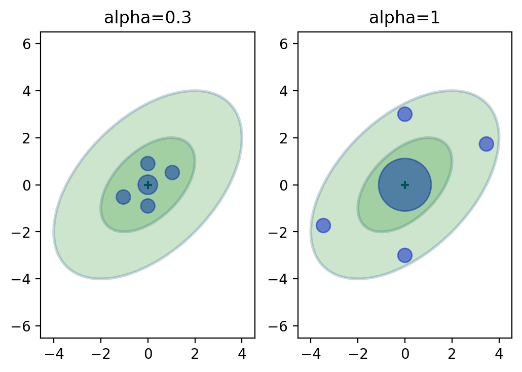
We can see that the sigma points lie between the first and second standard deviation, and that the larger \(\alpha\) spreads the points out.

Furthermore, the larger \(\alpha\) weights the mean (center point) higher than the smaller \(\alpha\), and weights the rest less.

This should fit our intuition - the further a point is from the mean the less we should weight it. We don’t know how these weights and sigma points are selected yet, but the choices look reasonable.

Sigma Point computation

The first sigma point is the mean of the input. This is the sigma point displayed in the center of the ellipses in the diagram above. We call this \(\mathcal X^0\).

\[\mathcal X^0 = \mu\]

We define \(\lambda = \alpha^2(n+\kappa)-n\) with \(n\) the dimension of \(\mu\), \(\alpha\) and \(\kappa\) being scaling parameters that determine how far the sigma points are spread from the mean.

The remaining sigma points are computed as:

\[\begin{split}\mathcal X^i = \begin{cases} \mu + \left( \sqrt{(n+\lambda)\Sigma}\right )_{i}& \text{for }i=1,\dots, n \\ \mu - \left( \sqrt{(n+\lambda)\Sigma}\right)_{i-n} &\text{for }i=(n+1),\dots, 2n \end{cases}\end{split}\]

\(i\) choose the \(i^th\) row vector of the matrix.

Weight Computation

This formulation uses one set of weights for the means, and another set for the covariance.

The weights for \(\mathcal X_0\) is computed as:

\[w^0_m = \frac{\lambda}{n+\lambda}\]

The weight for the covariance of \(\mathcal X_0\) is:

\[w^0_c = \frac{\lambda}{n+\lambda}+1-\alpha^2+\beta\]

For the other sigma points the weights are the same for the mean and covariance:

\[w_m^i = w_c^i = \frac{1}{2(n + \lambda)}, \quad i=1,2,\dots,2n\]

Important

Ordinarily these weights do not sum to one. Getting weights that sum to greater than one, or even negative values is expected.

Reasonable Choices for the Parameters

• \(\beta=2\) is a good choice for Gaussian problems,

• \(\kappa=3-n\) where \(n\) is the dimension of \(\mu\),

• and \(0 \le \alpha \le 1\) is an appropriate choice for \(\alpha\), where a larger value for \(\alpha\) spreads the sigma points further from the mean.

The Extended Kalman Filter

Contrary to the UKF, the Extended Kalman Filter (EKF) is not doing sampling to approximate the new estimate as a Gaussian.

The EKF handles nonlinearity by linearizing the system at the point of current estimate, then filter the linearized system.

Important

The EKF provides significant mathematical challenges, the most challenging filter you will see.

Linearizing the Kalman Filter

Remember that the Kalman Filter uses linear equations, so it does not work with nonlinear problems.

Problems can be nonlinear in two ways:

1. The process model might be non linear.

   • An object falling trough the atmosphere encounters drag which reduces its acceleration.

   • The drag coefficient varies based on the velocity of the object.

   • The resulting system is nonlinear.

2. The measurement could be nonlinear.

   • For example a radar gives a range and bearing to a target.

   • We use trigonometry, which is nonlinear, to compute the position of the target.

For the linear filter we have these equations for the process and measurement models:

\[\begin{split}\begin{aligned} x_t &= A_t x_{t-1} + B_t u_{t} + \epsilon_t \\ z_t &= C_t x_t + \delta_t\\ \end{aligned}\end{split}\]

For nonlinear model the linear expression \(A_t x_{t-1} + B_t u_{t}\) is replaced by a nonlinear function \(g(u, x)\), and the linear expression \(Cx\) is replaced by a non linear function \(h(x)\):

\[\begin{split}\begin{aligned} x_t &= g(u_t, x_{t-1}) + \epsilon_t\\ z_t &= h(x_t) + \delta_t \end{aligned}\end{split}\]

The EKF doesn’t alter the Kalman filter’s equations, it linearizes the nonlinear equations, then use the linear Kalman filter.

Example

Linearize means what it sounds like. We find a line that most closely matches the curve at a defined point. The graph below linearizes the parabola \(g(x)=x^2-2x\) at \(x=1.5\).

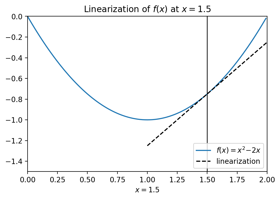
We linearize the systems by taking the derivative, which finds the slope of a curve:

\[\begin{split}\begin{aligned} g(x) &= x^2 - 2x\\ \frac{dg}{dx} &= 2x - 2 \end{aligned}\end{split}\]

and then evlauting it a \(x\):

\[\begin{split}\begin{aligned} m &= f(x=1.5)\\ &= 2(1.5) - 2\\ &= 1 \end{aligned}\end{split}\]

We can see it has a slope of 1.

Linearizing systems of differential equations is similar.

We linearize \(g(x,u)\) and \(h(x)\) by taking the partial derivatives of each to evaluate \(A\) and \(H\) at the point \(x_t\) and \(u_t\).

Note

We call the partial derivative of a matrix the Jacobian.

It gives us the discrete state transition matrix and measurement model matrix:

\[\begin{split}\begin{aligned} G &= {\frac{\partial{g(x_t, u_t)}}{\partial{x}}}\biggr|_{{x_t},{u_t}} \\ H &= \frac{\partial{h(\bar{x}_t)}}{\partial{\bar{x}}}\biggr|_{\bar{x}_t} \end{aligned}\end{split}\]

Written as Gaussian, the next state probability is approximated as follows:

\[\begin{split}\begin{aligned} p(x_t | u_t, x_{t-1}) &\approx\\ &\det(2\pi R_t)^{\frac{1}{2}}\exp\{ -\frac{1}{2}\left[x_t - g(u_t, \mu_{t-1}) - G_t(x_{t-1} - \mu_{t-1}) \right]^T\\ &R^{-1}_t \left[x_t - g(u_t, \mu_{t-1}) - G_t(x_{t-1} - \mu_{t-1}) \right] \} \end{aligned}\end{split}\]

Written as Gaussian, the next measurement probability is approximated as follows:

\[\begin{split}\begin{aligned} p(z_t | x_{t}) &\approx \det(2\pi Q_t)^{\frac{1}{2}}\exp\{ -\frac{1}{2}\left[z_t - h(\mu_{t}) - H_t(x_{t} - \mu_{t}) \right]^T\\ &Q^{-1}_t \left[z_t - h(\mu_{t}) - H_t(x_{t} - \mu_{t}) \right] \} \end{aligned}\end{split}\]

It leads to the following equations for the EKF. I put boxes around the differences from the linear filter.

\[\begin{split}\begin{array}{l|l} \text{linear Kalman filter} & \text{EKF} \\ \hline & \boxed{ G = {\frac{\partial{g(x_t, u_t)}}{\partial{x}}}\biggr|_{{x_t},{\mathbf u_t}}} \\ \bar \mu = A\mu + Bu & \boxed{\bar \mu = g(x, u)} \\ \bar \Sigma = A\Sigma A^T+ R & \bar \Sigma = G\Sigma G^T+R \\ \hline & \boxed{ H = \frac{\partial{h(\bar{x}_t)}}{\partial{\bar{x}}}\biggr|_{\bar{x}_t}} \\ y = z - H \bar\mu & y = z - \boxed{h(\bar\mu)}\\ K = \bar\Sigma H^T (H\bar\Sigma H^T + Q)^{-1} & K = \bar\Sigma H^T (H\bar\Sigma H^T + Q)^{-1} \\ \mu=\bar\mu +Ky & x=\bar\mu +Ky \\ \Sigma= (I-KH)\bar\Sigma & \Sigma= (I-KH)\bar\Sigma \end{array}\end{split}\]

Note that we don’t use \(G\mu\) to propagate the state for the EKF as the linearization causes inaccuracies.

It is typical to compute \(\bar\mu\) using a suitable numerical integration technique such as Euler.

This is why we user \(g(\mu, u)\) and \(h(\bar\mu)\).

Usually, you’re lost at this point, so we will do an example to understand.

Example: Tracking an Aircraft

In this example we are trying to tracks an airplane using ground based radar (again…).

To give you some context:

• Radars work by emitting a beam of radio waves and scanning for a return bounce.

• Anything in the beam’s path will reflects some of the signal back to the radar.

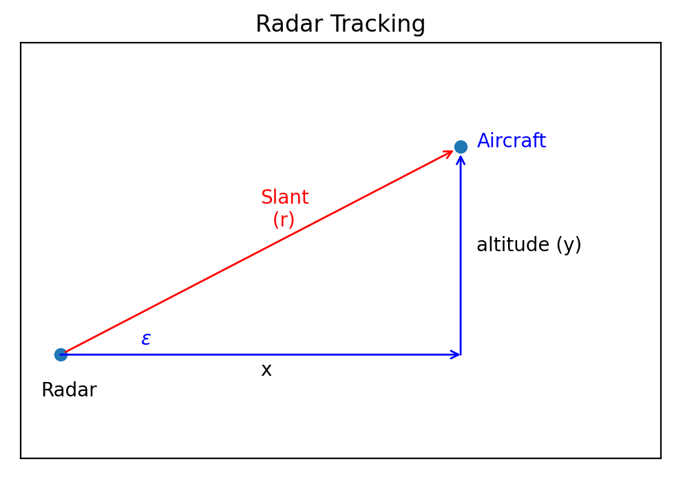
• By timing how long it takes for the reflected signal to get back to the radar the system can compute the slant distance - the straight line distance from the radar installation to the object.

The relationship between the radar’s slant range distance \(r\) and elevation angle \(\epsilon\) with the horizontal position \(x\) and altitude \(y\) of the aircraft is illustrated in the figure below:

Designing the State Variables

We want to track the position of an aircraft assuming a constant velocity and altitude, and measurements of the slant distance to the aircraft.

Meaning we need 3 variables:

• horizontal distance

• horizontal velocity

• altitude

\[\begin{split}\mu = \begin{bmatrix}\mathtt{distance} \\\mathtt{velocity}\\ \mathtt{altitude}\end{bmatrix}= \begin{bmatrix}x \\ \dot x\\ y\end{bmatrix}\end{split}\]

Designing the Process Model

We assume a newtonian, kinematic system for the aircraft:

\[\begin{split}A = \left[\begin{array}{cc|c} 1 & \Delta t & 0\\ 0 & 1 & 0 \\ \hline 0 & 0 & 1\end{array}\right]\end{split}\]

The matrix is partioned into blocks to show the upper left block is a constant velocity and the lower right block is a constant position.

However, it is important for you to learn how to find these matrices.

Remember, that we model systems with a set of differential equations, basically we need an equation in the form of:

\[Fx + \epsilon\]

where \(\epsilon\) is the system noise.

The variable \(x\) and \(y\) are independent, so we can compute them separately.

The differantial equations for motion in one dimension are:

\[\begin{split}\begin{aligned} v &= \dot x \\ a &= \ddot{x} = 0 \end{aligned}\end{split}\]

Now we put the differential equations into state-space form.

Note

If this was a second or greater order differential system we would have to first reduce them to an equivalent set of first degree equations.

The equations are first order, so we put them in state space matrix form as

\[\begin{split}\begin{aligned} \begin{bmatrix}\dot x \\ \ddot{x}\end{bmatrix} &= \begin{bmatrix}0&1\\0&0\end{bmatrix} \begin{bmatrix}x \\ \dot x\end{bmatrix} \\ \dot x &= Fx \end{aligned}\end{split}\]

where \(F=\begin{bmatrix}0&1\\0&0\end{bmatrix}\).

Recall that \(F\) is the system dynamics matrix.

It describes a set of linear differential equations. From it we must compute the state transition matrix \(A\).

\(A\) describes a discrete set of linear equations which compute \(x\) for a discrete time step \(\Delta t\).

A common way to compute \(A\) is to use the power series expansion of the matrix exponential:

\[A(\Delta t) = e^{F\Delta t} = I + F\Delta t + \frac{( F\Delta t)^2}{2!} + \frac{(F \Delta t)^3}{3!} + \dots\]

\(F^2 = \begin{bmatrix}0&0\\0&0\end{bmatrix}\), so all higher powers of \(F\) are also \(0\). Thus the power series expansion is:

\[\begin{split}\begin{aligned} A &=I + F\Delta t + 0 \\ &= \begin{bmatrix}1&0\\0&1\end{bmatrix} + \begin{bmatrix}0&1\\0&0\end{bmatrix}\Delta t\\ A &= \begin{bmatrix}1&\Delta t\\0&1\end{bmatrix} \end{aligned}\end{split}\]

This is the same result used by the kinematic equations!

Designing the Measurement Model

The measurement function takes the state estimate of the prior \(\bar x\) and turn it into a measurement of the slant range distance.

We use the Pythagorean theorem to derive:

\[h(\bar \mu) = \sqrt{x^2 + y^2}\]

The relationship between the slant distance and the position on the ground is nonlinear due to the square root.

We linearize it by evaluating its partial derivative at \(\mu_t\):

\[H = \frac{\partial{h(\bar \mu)}}{\partial{\bar \mu}}\biggr|_{\bar \mu_t}\]

The partial derivative of a matrix is called a Jacobian, and takes the form

\[\begin{split}\frac{\partial H}{\partial \bar \mu} = \begin{bmatrix} \frac{\partial h_1}{\partial x_1} & \frac{\partial h_1}{\partial x_2} &\dots \\ \frac{\partial h_2}{\partial x_1} & \frac{\partial h_2}{\partial x_2} &\dots \\ \vdots & \vdots \end{bmatrix}\end{split}\]

In other words, each element in the matrix is the partial derivative of the function \(h\) with respect to the \(x\) variables.

For our problem we have

\[H = \begin{bmatrix}{\partial h}/{\partial x} & {\partial h}/{\partial \dot{x}} & {\partial h}/{\partial y}\end{bmatrix}\]

Solving each in turn:

\[\begin{split}\begin{aligned} \frac{\partial h}{\partial x} &= \frac{\partial}{\partial x} \sqrt{x^2 + y^2} \\ &= \frac{x}{\sqrt{x^2 + y^2}} \end{aligned}\end{split}\]

and

\[\begin{split}\begin{aligned} \frac{\partial h}{\partial \dot{x}} &= \frac{\partial}{\partial \dot{x}} \sqrt{x^2 + y^2} \\ &= 0 \end{aligned}\end{split}\]

and

\[\begin{split}\begin{aligned} \frac{\partial h}{\partial y} &= \frac{\partial}{\partial y} \sqrt{x^2 + y^2} \\ &= \frac{y}{\sqrt{x^2 + y^2}} \end{aligned}\end{split}\]

giving us

\[H = \begin{bmatrix} \frac{x}{\sqrt{x^2 + y^2}} & 0 & & \frac{y}{\sqrt{x^2 + y^2}} \end{bmatrix}\]

This may seem complicated, so step back and recognize that all of this math is doing something very simple.

• We have an equation for the slant range to the airplane which is nonlinear.

• The Kalman filter only works with linear equations, so we need to find a linear equation that approximates \(H\).

Finding the slope of a nonlinear equation at a given point is a good approximation.

For the Kalman filter, the ‘given point’ is the state variable \(\mu\) so we need to take the derivative of the slant range with respect to \(\mu\).

For the linear Kalman filter \(H\) was a constant that we computed prior to running the filter.

For the EKF \(H\) is updated at each step as the evaluation point \(\bar \mu\) changes at each epoch.

Let’s now write a Python function that computes the Jacobian of \(h\) for this problem.

Activity

1. Implement the function calculating the Jacobian of h.

from math import sqrt
def HJacobian_at(x):
    """
    Compute jacobian.
    """

2. Implement the measurement function.

from math import sqrt
def hx(x):
    """
    Compute measurement.
    """

Design the Process and Measurement Noise

The radar measures the range to a target.

We will use \(\sigma_{range}= 5\) meters for the noise.

This gives us

\[Q = \begin{bmatrix}\sigma_{range}^2\end{bmatrix} = \begin{bmatrix}25\end{bmatrix}\]

The design of \(R\) requires some discussion.

The state \(\mu= \begin{bmatrix}x & \dot x & y\end{bmatrix}^T\).

The first two elements are position (down range distance) and velocity.

The third element of \(\mu\) is altitude, which we are assuming is independent of the down range distance.

That leads us to a block design of \(R\) of:

\[\begin{split}R = \begin{bmatrix}R_\mathtt{x} & 0 \\ 0 & R_\mathtt{y}\end{bmatrix}\end{split}\]