Topic 4 - Discrete Bayes Filters

Introduction

Sensors are noisy. The world is full of data and events that we want to measure and track, but we cannot rely on sensors to give us perfect information.

• The GPS in my car reports altitude. Each time I pass the same point in the road it reports a slightly different altitude.

• My kitchen scale gives me different readings if I weigh the same object twice.

In simple cases the solution is obvious.

• If my scale gives slightly different readings, I can just take a few readings and average them.

• Or I can replace it with a more accurate scale.

What can we do when the sensors are very noisy? Or if it’s hard to take multiple measurements?

• We may be trying to track the movement of a low-flying aircraft.

• We may want to create an autopilot for a drone.

We will see different algorithms, but they are all based on Bayesian probability. In simple terms Bayesian probability determines what is likely to be true based on past information.

Example

• If I asked you the heading of my car at this moment, you would have no idea.

• You’d proffer a number between \(1^\circ\) and \(360^\circ\) degrees, and have a 1 in 360 chance of being right.

• Now suppose I told you that 2 seconds ago its heading was \(243^\circ\). In 2 seconds my car could not turn very far so you could make a far more accurate prediction. You are using past information to more accurately infer information about the present or future.

We discussed the fact that the world is also noisy.

• I may have just braked for a dog or swerved around a pothole.

• Strong winds and ice on the road are external influences on the path of my car.

Important

In robotics literature we call this noise though you may not think of it that way.

SciPy, NumPy, and Matplotlib

Most of the examples and codes that I will provide will be in Python using these three libraries.

If you’re not familiar with them, I recommend taking a look at them on your own time.

To make sure you can follow, I give you a quick reminder.

You can create arrays with numpy very easily:

import numpy as np

x = np.array([1, 2, 3])

We can also create nested arrays as easily:

x = np.array([[1, 2, 3],
          [4, 5, 6]])

By default the arrays use the data type of the values in the list;if there are multiple types then it will choose the type that most accurately represents all the values.

So, for example, if your list contains a mix of int and float the data type of the array would be of type float. You can override this with the dtype parameter.

x = np.array([1, 2, 3], dtype=float)

You can perform matrix addition with the + operator, but matrix multiplication requires the dot method or function.

The * operator performs element-wise multiplication, which is not what you want for linear algebra.

x = np.array([[1., 2.],
          [3., 4.]])
print('addition:\n', x + x)
print('\nelement-wise multiplication\n', x * x)
print('\nmultiplication\n', np.dot(x, x))
print('\ndot is also a member of np.array\n', x.dot(x))

The results would be:

addition:
[[2. 4.]
[6. 8.]]

element-wise multiplication
[[ 1.  4.]
[ 9. 16.]]

multiplication
[[ 7. 10.]
[15. 22.]]

Python 3.5 introduced the @ operator for matrix multiplication.

x @ x

Giving:

array([[ 7., 10.],
    [15., 22.]])

You can get the transpose with .T, and the inverse with numpy.linalg.inv. The SciPy package also provides the inverse function.

import scipy.linalg as linalg

print('transpose\n', x.T)
print('\nNumPy ninverse\n', np.linalg.inv(x))
print('\nSciPy inverse\n', linalg.inv(x))

Discrete Bayes Filter

Now, It’s time to speak about our first filter, the Discrete Bayes Filter. We saw a very simplified version in the previous topic.

To go further, we will consider that the computer science department has a dog called Alan.

It’s a good dog, but he tends to wander out of offices and down the halls, so we need a way to track him in real time.

So during a hackathon somebody invented a sonar sensor to attach to the dog’s collar.

It emits a signal, listens for the echo, and based on how quickly an echo comes back we can tell whether the dog is in front of an open doorway or not.

It also senses when the dog walks, and reports in which direction the dog has moved. It connects to the network via wifi and sends an update once a second.

Problem representation

We will consider a simplified problem with only 10 positions in a hallway, number from 0 to 9.

For different reasons, we will consider that the hallway is circular, so when you move to the right from position 9 you come back to position 0.

In a robotic application, you do not have any reason to believe that the dog is in any specific position at the beginning of the mission.

There are 10 positions, so the probability that he is in any given position is 1/10.

import numpy as np
belief = np.array([1/10]*10)
print(belief)

[0.1 0.1 0.1 0.1 0.1 0.1 0.1 0.1 0.1 0.1]

This is our initial belief, before taking any measurement.

Now we can create the map of the hallway. We will use 1 for doors and 0 for walls.

hallway = np.array([1, 1, 0, 0, 0, 0, 0, 0, 1, 0])

You start listening to Alan’s transmissions on the network, and the first data you get from the sensor is door.

• For the moment assume the sensor always returns the correct answer.

• From this you conclude that he is in front of a door, but which one?

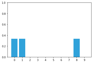
• You have no reason to believe he is in front of the first, second, or third door.

• All doors are equally likely, and there are three of them, so you assign a probability of 1/3 to each door.

belief = np.array([1/3, 1/3, 0, 0, 0, 0, 0, 0, 1/3, 0])

Giving us:

Suppose we were to read the following from Alan’s sensor:

• door

• move right

• door

Activity

Can you deduce Alan’s location?

I designed the hallway layout and sensor readings to give us an exact answer quickly.

Noisy Sensors

Perfect sensors are rare.

Perhaps the sensor would not detect a door if Alan sat in front of it while scratching himself, or misread if he is not facing down the hallway.

Thus when you get door you cannot use \(1/3\) as the probability.

You have to assign less than \(1/3\) to each door, and assign a small probability to each blank wall position. Something like:

[.31, .31, .01, .01, .01, .01, .01, .01, .31, .01]

Obviously, we need to do that correctly.

What we want is to have a belief and calculate the updated belief ( or posterior):

\[\mathtt{posterior} = \frac{\mathtt{likelihood} \times \mathtt{prior}}{\mathtt{normalization}}\]

If you don’t remember check the previous topic.

Computation of the likelihood varies per problem. For example, the sensor might not return just 1 or 0, but a float between 0 and 1 indicating the probability of being in front of a door.

To make it more general, we will include a parameter in our function that will give the probability that the measurement is correct.

def lh_hallway(hall, z, z_prob):
    """ compute likelihood that a measurement matches
    positions in the hallway."""

    try:
        scale = z_prob / (1. - z_prob)
    except ZeroDivisionError:
        scale = 1e8

    likelihood = np.ones(len(hall))
    likelihood[hall==z] *= scale
    return likelihood

Now that we have a way to calculate the likelihood, we can create te update function:

def normalize(belief):
    return belief / sum(belief)

def update(likelihood, prior):
    return normalize(likelihood * prior)

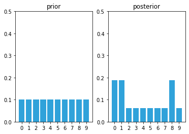
If we test it, with the measurement door with a probability of 0.75:

belief = np.array([0.1] * 10)
likelihood = lh_hallway(hallway, z=1, z_prob=.75)
update(likelihood, belief)

array([0.188, 0.188, 0.062, 0.062, 0.062, 0.062, 0.062, 0.062, 0.188, 0.062])

Activity

What happens if we have the measurement door, but with a probability of 0.3?

Incorporating movement

Recall how quickly we were able to find an exact solution when we incorporated a series of measurements and movement updates.

However, that occurred in a fictional world of perfect sensors. Might we be able to find an exact solution with noisy sensors?

Unfortunately, the answer is no.

Even if the sensor readings perfectly match an extremely complicated hallway map, we cannot be 100% certain that the dog is in a specific position - there is, after all, a tiny possibility that every sensor reading was wrong!

First let’s deal with the simple case - assume the movement sensor is perfect, and it reports that the dog has moved one space to the right. How would we alter our belief array?

I hope that after a moment’s thought it is clear that we should shift all the values one space to the right.

def perfect_predict(belief, move):
    """ move the position by `move` spaces, where positive is
    to the right, and negative is to the left
    """
    n = len(belief)
    result = np.zeros(n)
    for i in range(n):
        result[i] = belief[(i-move) % n]
    return result

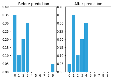
# Initial belief
belief = np.array([.35, .1, .2, .3, 0, 0, 0, 0, 0, .05])

# Belief after update
belief = perfect_predict(belief, 1)

Adding Uncertainty to the Prediction

perfect_predict() assumes perfect measurements, but all sensors have noise.

What if the sensor reported that our dog moved one space, but he actually moved two spaces, or zero?

Assume that the sensor’s movement measurement is 80% likely to be correct, 10% likely to overshoot one position to the right, and 10% likely to undershoot to the left.

That is, if the movement measurement is 4 (meaning 4 spaces to the right), the dog is 80% likely to have moved 4 spaces to the right, 10% to have moved 3 spaces, and 10% to have moved 5 spaces.

Let’s try coding that:

def predict_move(belief, move, p_under, p_correct, p_over):
    n = len(belief)
    prior = np.zeros(n)
    for i in range(n):
        prior[i] = (
            belief[(i-move) % n]   * p_correct +
            belief[(i-move-1) % n] * p_over +
            belief[(i-move+1) % n] * p_under)
    return prior

If we apply:

belief = [0., 0., 0., 1., 0., 0., 0., 0., 0., 0.]
prior = predict_move(belief, 2, .1, .8, .1)

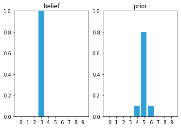
It seems to work, Alan has 10% chance of being in location 4 and 10% in being in location 6.

Warning

It’s a prior, so a prediction! It’s something you can calculate before confirming that the agent has done this action.

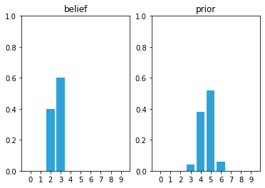
What happens if the initial belief is not 100% certain?

belief = [0, 0, .4, .6, 0, 0, 0, 0, 0, 0]
prior = predict_move(belief, 2, .1, .8, .1)

array([0.  , 0.  , 0.  , 0.04, 0.38, 0.52, 0.06, 0.  , 0.  , 0.  ])

Activity

Try to change the initial belief and movements and see if you can calculate the probabilities manually.

It is important that you understand the calculation behind.

After performing the update the probabilities are not only lowered, but they are strewn out across the map.

This is not a coincidence, or the result of a carefully chosen example - it is always true of the prediction.

If the sensor is noisy we lose some information on every prediction.

Important

Suppose we were to perform the prediction an infinite number of times. What would the result be?

If we lose information on every step, we must eventually end up with no information at all, and our probabilities will be equally distributed across the belief array.

Here is an example after 100 iterations.

Generalizing with Convolution

We made the assumption that the movement error is at most one position. But it is possible for the error to be two, three, or more positions. As programmers we always want to generalize our code so that it works for all cases.

This is easily solved with convolution. Convolution modifies one function with another function. In our case we are modifying a probability distribution with the error function of the sensor. The implementation of predict_move() is a convolution, though we did not call it that. Formally, convolution is defined as

\[(f \ast g) (t) = \int_0^t \!f(\tau) \, g(t-\tau) \, \mathrm{d}\tau\]

where \(f\ast g\) is the notation for convolving f by g. It does not mean multiply.

Integrals are for continuous functions, but we are using discrete functions. We replace the integral with a summation, and the parenthesis with array brackets.

\[(f \ast g) [t] = \sum\limits_{\tau=0}^t \!f[\tau] \, g[t-\tau]\]

Comparison shows that predict_move() is computing this equation - it computes the sum of a series of multiplications.

Khan Academy has a good introduction to convolution, and Wikipedia has some excellent animations of convolutions.

But the general idea is already clear. You slide an array called the kernel across another array, multiplying the neighbours of the current cell with the values of the second array.

In our example above we used 0.8 for the probability of moving to the correct location, 0.1 for undershooting, and 0.1 for overshooting. We make a kernel of this with the array [0.1, 0.8, 0.1].

All we need to do is write a loop that goes over each element of our array, multiplying by the kernel, and summing up the results. To emphasize that the belief is a probability distribution I have named it pdf.

SciPy provides a convolution routine, convolve() in the ndimage.filters module. We need to shift the pdf by offset before convolution; np.roll() does that. The move and predict algorithm can be implemented with one line.

def predict(pdf, offset, kernel, mode='wrap', cval=0.):

    if mode == 'wrap':
        return convolve(np.roll(pdf, offset), kernel, mode='wrap')

    return convolve(shift(pdf, offset, cval=cval), kernel,
                    cval=cval, mode='constant')

Integrating Measurements and Movement updates

The problem of losing information during a prediction may make it seem as if our system would quickly devolve into having no knowledge.

However, each prediction is followed by an update where we incorporate the measurement into the estimate.

The update improves our knowledge. The output of the update step is fed into the next prediction.

The prediction degrades our certainty. That is passed into another update, where certainty is again increased.

Taking back our first example.

hallway = np.array([1, 1, 0, 0, 0, 0, 0, 0, 1, 0])
prior = np.array([.1] * 10)
likelihood = lh_hallway(hallway, z=1, z_prob=.75)
posterior = update(likelihood, prior)

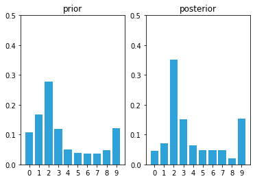
After the first update we have assigned a high probability to each door position, and a low probability to each wall position.

kernel = (.1, .8, .1)
prior = predict(posterior, 1, kernel)

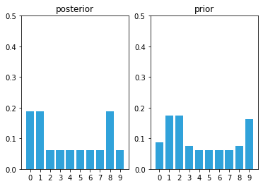
The predict step shifted these probabilities to the right, smearing them about a bit. Now let’s look at what happens at the next sense.

likelihood = lh_hallway(hallway, z=1, z_prob=.75)
posterior = update(likelihood, prior)

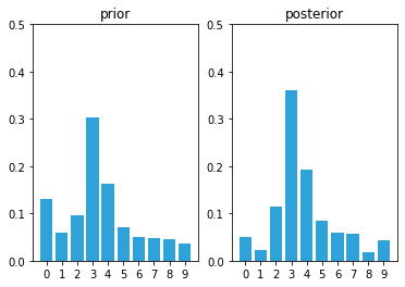
Notice the tall bar at position 1. This corresponds with the (correct) case of starting at position 0, sensing a door, shifting 1 to the right, and sensing another door. No other positions make this set of observations as likely. Now we will add an update and then sense the wall.

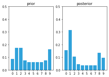
prior = predict(posterior, 1, kernel)
likelihood = lh_hallway(hallway, z=0, z_prob=.75)
posterior = update(likelihood, prior)

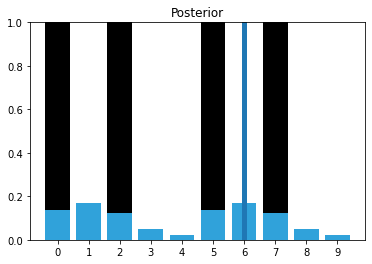
This is exciting! We have a very prominent bar at position 2 with a value of around 35%. It is over twice the value of any other bar in the plot, and is about 4% larger than our last plot, where the tallest bar was around 31%. Let’s see one more cycle.

prior = predict(posterior, 1, kernel)
likelihood = lh_hallway(hallway, z=0, z_prob=.75)
posterior = update(likelihood, prior)

The Discrete Bayes Algorithm

Finally, we can talk about the algorithm itself!

This figure illustrates the algorithm:

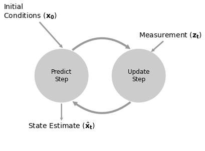
Mathematicaly we calculate the filter with the following equations:

\[\begin{split}\begin{aligned} \bar {\mathbf x} &= \mathbf x \ast f_{\mathbf x}(\bullet)\, \, &\text{Predict Step} \\ \mathbf x &= \|\mathcal L \cdot \bar{\mathbf x}\|\, \, &\text{Update Step}\end{aligned}\end{split}\]

where \(\bar{x}\) is the predicted state and \(\mathcal L\) is the likelihood function.

The \(\|\|\) notation denotes taking the norm.

We need to normalize the product of the likelihood with the prior to ensure \(x\) is a probability distribution that sums to one.

We can express this in pseudocode.

Initialization

1. Initialize our belief in the state

Predict

1. Based on the system behaviour, predict state for the next time step

2. Adjust belief to account for the uncertainty in prediction.

Update

1. Get a measurement and associated belief about its accuracy

2. Compute how likely it is the measurement matches each state

3. Update state belief with this likelihood.

Algorithms in this form are sometimes called predictor correctors. We make a prediction, then correct them.

Activity

Create a function discrete_bayes_sim(prior, kernel, measurements, z_prob, hallway) that has parameters:

• prior: The initial prior

• kernel: the kernel

• measurement: a list of measurements

• z_prob: the probability that the measurement is accurate.

• hallway: the hallway

Try it with z_prob=1.

The Effect of Bad Sensor Data

You may be suspicious of the results above because we always passed correct sensor data into the functions.

However, we are claiming that this code implements a filter - it should filter out bad sensor measurements. Does it do that?

To make this easy to program and visualize I will change the layout of the hallway to mostly alternating doors and hallways, and run the algorithm on 6 correct measurements:

hallway = np.array([1, 0, 1, 0, 0]*2)
kernel = (.1, .8, .1)
prior = np.array([.1] * 10)
zs = [1, 0, 1, 0, 0, 1]
z_prob = 0.75
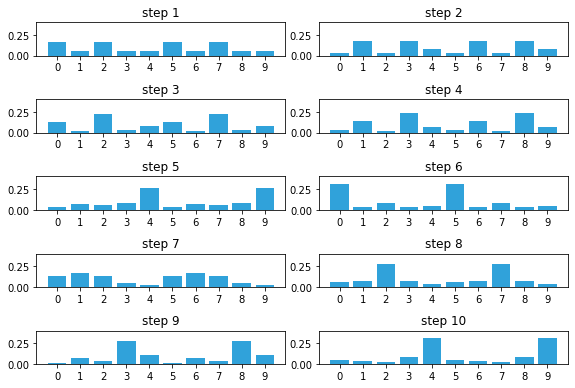
priors, posteriors = discrete_bayes_sim(prior, kernel, zs, z_prob, hallway)

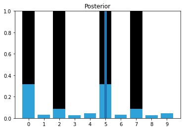
We have identified the likely cases of having started at position 0 or 5, because we saw this sequence of doors and walls: 1,0,1,0,0.

Now I inject a bad measurement. The next measurement should be 0, but instead we get a 1:

measurements = [1, 0, 1, 0, 0, 1, 1]
priors, posteriors = discrete_bayes_sim(prior, kernel, measurements, z_prob, hallway)

That one bad measurement has significantly eroded our knowledge. Now let’s continue with a series of correct measurements.

measurements = [1, 0, 1, 0, 0, 1, 1, 1, 0, 0]

Drawbacks and Limitations

Do not be mislead by the simplicity of the examples I chose.

This is a robust and complete filter, and you may use the code in real-world solutions. If you need a multimodal, discrete filter, this filter works.

With that said, this filter it is not used often because it has several limitations.

1. The filter does not scale well.

   • Our dog tracking problem used only one variable, \(pos\), to denote the dog’s position.

   • Most interesting problems will want to track several things in a large space. Realistically, at a minimum we would want to track our dog’s \((x,y)\) coordinate, and probably his velocity \((\dot{x},\dot{y})\) as well.

   • We have not covered the multidimensional case, but instead of an array we use a multidimensional grid to store the probabilities at each discrete location.

   • Each update() and predict() step requires updating all values in the grid, so a simple four variable problem would require \(O(n^4)\) running time per time step.

   • Realistic filters can have 10 or more variables to track, leading to exorbitant computation requirements.

2. The filter is discrete, but we live in a continuous world.

   • The histogram requires that you model the output of your filter as a set of discrete points.

   • It gets exponentially worse as we add dimensions. A 100x100 \(m^2\) courtyard requires 100,000,000 bins to get 1cm accuracy.

3. The filter is multimodal.

   • In the last example we ended up with strong beliefs that the dog was in position 4 or 9. This is not always a problem.

   • But imagine if the GPS in your car reported to you that it is 40% sure that you are on D street, and 30% sure you are on Willow Avenue.

4. A forth problem is that it requires a measurement of the change in state.

   • We need a motion sensor to detect how much the dog moves.

Important

It is a good solution for simple problems!