Lab 4 - Implementing the EKF

In this lab, you will continue the example started in topic 7.

The idea is to track an airplane with a radar.

I am giving you the radar simulator.

from numpy.random import randn
import math

class RadarSim:
    """ Simulates the radar signal returns from an object
    flying at a constant altityude and velocity in 1D.
    """

    def __init__(self, dt, pos, vel, alt):
        self.pos = pos
        self.vel = vel
        self.alt = alt
        self.dt = dt

    def get_range(self):
        """ Returns slant range to the object. Call once
        for each new measurement at dt time from last call.
        """

        # add some process noise to the system
        self.vel = self.vel  + .1*randn()
        self.alt = self.alt + .1*randn()
        self.pos = self.pos + self.vel*self.dt

        # add measurement noise
        err = self.pos * 0.05*randn()
        slant_dist = math.sqrt(self.pos**2 + self.alt**2)

        return slant_dist + err

Implementing the EKF

Remember the equations for the EKF:

\[\begin{split}\begin{array}{l|l} \text{linear Kalman filter} & \text{EKF} \\ \hline & \boxed{ G = {\frac{\partial{g(x_t, u_t)}}{\partial{x}}}\biggr|_{{x_t},{\mathbf u_t}}} \\ \bar \mu = A\mu + Bu & \boxed{\bar \mu = g(x, \mu)} \\ \bar \Sigma = A\Sigma A^T+ R & \bar \Sigma = G\Sigma G^T+R \\ \hline & \boxed{ H = \frac{\partial{h(\bar{x}_t)}}{\partial{\bar{x}}}\biggr|_{\bar{x}_t}} \\ y = z - H \bar\mu & y = z - \boxed{h(\bar\mu)}\\ K = \bar\Sigma H^T (H\bar\Sigma H^T + Q)^{-1} & K = \bar\Sigma H^T (H\bar\Sigma H^T + Q)^{-1} \\ \mu=\bar\mu +Ky & x=\bar\mu +Ky \\ \Sigma= (I-KH)\bar\Sigma & \Sigma= (I-KH)\bar\Sigma \end{array}\end{split}\]

Predict

Create a function predict. Remember that in this example, the transition function is linear.

def predict(A, mu, Sigma, R):
    """ Your code """
    return mu, Sigma

Update

You need to update the prediction with the new measurement. In this case the measurement function is nonlinear. So you need to use both the nonlinear measurement function, and the jacobian function.

def update(mu, Sigma, H, h, z, Q):
    """ Your code """
    return mu, Sigma

H represent the jacobian calculated for mu (so not the function directly, the result) and h the nonlinear function.

You can use the function we have done in topic 7.

Using the EKF

The noise

We need to define the process noise and the measurement noise.

I am giving you this part:

from filterpy.common import Q_discrete_white_noise

range_std = 5. # meters
Q = np.diag([range_std**2])
R = np.zeros((3,3))
R[0:2, 0:2] = Q_discrete_white_noise(2, dt=dt, var=0.1)
R[2,2] = 0.1

Putting everything together

You should be able to run the following code to test your filter.

from numpy.core import multiarray

dt = 0.05
radar = RadarSim(dt, pos=0., vel=100., alt=1000.)

mu = np.array([radar.pos-100, radar.vel+100, radar.alt+1000])
Sigma = np.eye(3)*50

A = np.eye(3) + np.array([[0, 1, 0],
                [0, 0, 0],
                [0, 0, 0]])*dt

mus, track = [], []
for i in range(int(20/dt)):
    z = radar.get_range()
    track.append((radar.pos, radar.vel, radar.alt))

    H = HJacobian_at(mu)
    mu, Sigma = update(mu, Sigma, H, h, np.array([z]), Q)
    mus.append(mu)
    mu, Sigma = predict(A, mu, Sigma, R)

mus = np.asarray(mus)
track = np.asarray(track)
time = np.arange(0, len(mus)*dt, dt)
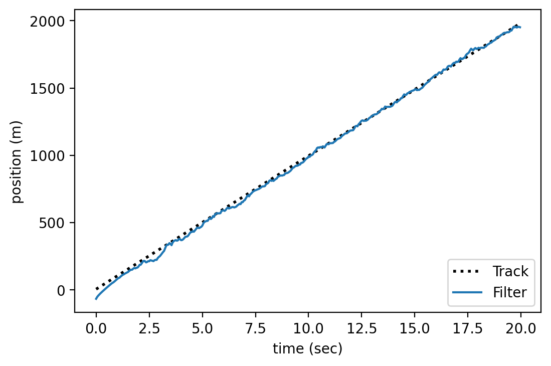
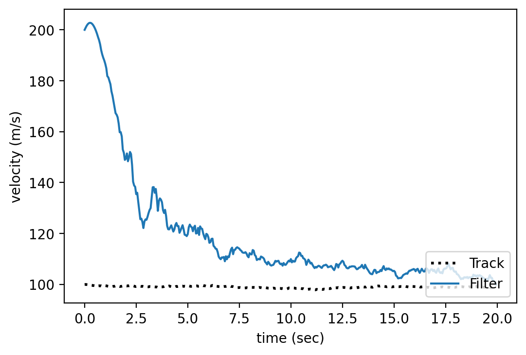
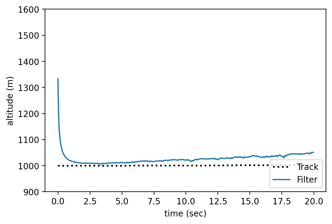
plot_radar(mus, track, time)

The code for the plot is given below:

+ show/hide code

If eveyrthing works then you should obtain something very similar: