13. Partially Observable Markov Decision Process

  • Markov Decision Processe (MDP) is a good framework for control decision when the measurement is perfect.

  • However, most of the time the measurement is not perfect.

  • To address the uncertainty on the measurement a new framework was created: Partially Observable Markov Decision Process (POMDP)

13.1. How does it work?

  • In MDPs, we use the value iteration function:

\[v^*_\pi(s) = \max_a \sum_{s'}p(s'|s,a)\left[ r(s,a) + \gamma v^*(s') \right]\]
  • However, in POMDPs we don’t know what the state \(s\) is.

  • In robotics we use the notion of belief state \(b\).

  • If we replace \(s\) by \(b\) in the previous equation we obtain:

\[v^*_\pi(b) = \max_a \int_{b'}p(b'|b,a)\left[ r(b,a) + \gamma v^*(b') db'\right]\]
  • Giving us the control policy:

\[\pi(b) = \arg\max_a \int_{b'}p(b'|b,a)\left[ r(b,a) + \gamma v^*(b') db'\right]\]
  • The issue with using the belief state is that it is continuous.

Important

When the state space, the action space, the space of observations and the planning horizon are all finite there is a solution.

Example

  • We will consider the following problem represented as a POMDP.

../../_images/two_states_pomdp.drawio.png

  • The actions \(u_1\) and \(u_2\) are giving different rewards depending of the states.

  • Only \(u_3\) is giving the same one: \(-1\).

  • The goal of the robot is to use \(u_3\) to gain information of the real state.

13.1.1. Action selection

  • Before solving the problem we need to have a way to calculate the reward for a specific action.

  • For any belief state \(b = (p_1, p_2)\), the expected reward us calculated as:

\[r(b, u) = \mathbb{E}\left[ r(s, u) \right] = p_1\times r(s_1, u) + p_2\times r(s_2, u)\]
  • which gives use the following expected rewards:
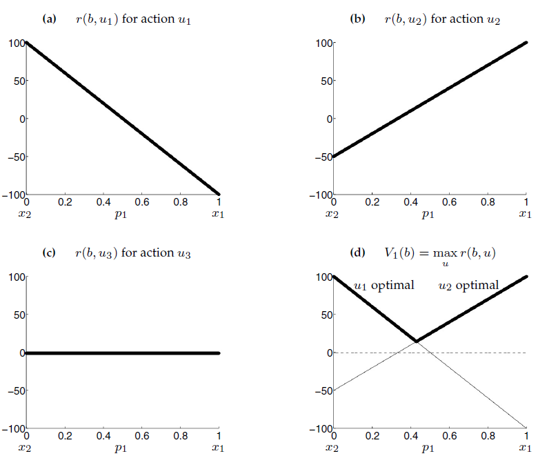
../../_images/pomdp_belief_reward.png

Important

Even with two states calculating the expected reward is complex.

Also the we can see the expected value function is piecewise linear and convex!

Activity

  • Calculate the expected reward for the following belief states and every actions:

    • \(b_1 = (0.3, 0.7)\)

    • \(b_2 = (0.5, 0.5)\)

    • \(b_3 = (0.7, 0.3)\)

  • Calculating the best action at one time step is solving a set of linear equations:

\[\begin{split}\begin{aligned} v_1(b) &= \max_{u}r(b,u)\\ &= \max \begin{Bmatrix} -100p_1 & +100(1-p_1) \\ 100p_1 & -50(1-p_1)\\ -1 \end{Bmatrix} \end{aligned}\end{split}\]
  • As only the first two linear functions contribute to the optimal action we can prune the third one:

\[\begin{split}v_1(b) &= \max \begin{Bmatrix} -100p_1 & +100(1-p_1) \\ 100p_1 & -50(1-p_1)\\ \end{Bmatrix}\end{split}\]

Note

Prunable functions are usually represented by dashed lines.
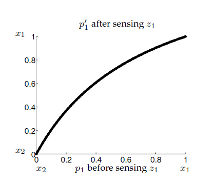
13.1.2. Sensing

  • We suppose now that we receive a measurement \(z_1\).

  • We can apply Bayes rule:

    • For \(p_1\):

    \[\begin{split}\begin{aligned} p_1' &= p(x_1|z)\\ &= \frac{p(z_1|x_1)p(x_1)}{p(z_1)}\\ &= \frac{0.7p_1}{p(z_1)} \end{aligned}\end{split}\]
    • For \(p_2\):

    \[\begin{aligned} p_2' &= \frac{0.3(1-p_1)}{p(z_1)} \end{aligned}\]
  • The only issue is the normalizer \(p(z_1)\):

\[p(z_1) = 0.7p_1 + 0.3(1-p_1) = 0.4p_1 + 0.3\]
  • If we use the measurement, our belief becomes nonlinear:

../../_images/sensing_01.png

  • Changing the expected value:
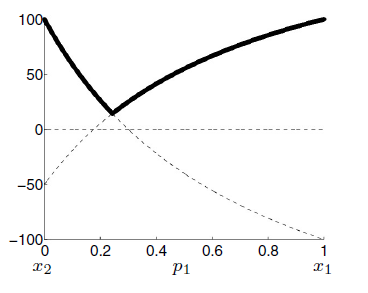
../../_images/sensing_02.png

  • Mathematically:

\[\begin{split}\begin{aligned} v_1(b|z_1) &= \max \begin{Bmatrix} -100p_1' & +100p_2' \\ 100p_1' & +-50p_2'\\ \end{Bmatrix}\\[10pt] &= \max \begin{Bmatrix} -100\frac{0.7p_1}{p(z_1)} & +100\frac{0.3(1-p_1)}{p(z_1)} \\ 100\frac{0.7p_1}{p(z_1)} & -50\frac{0.3(1-p_1)}{p(z_1)}\\ \end{Bmatrix}\\[10pt] &= \frac{1}{p(z_1)}\max \begin{Bmatrix} -70p_1 & +30(1-p_1) \\ 70p_1 &-15(1-p_1)\\ \end{Bmatrix}\\ \end{aligned}\end{split}\]
  • This is only considering one measurement.

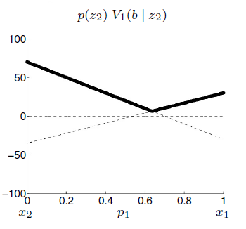
  • We need to calculate the value before sensing for every measurement:

\[\bar{v_1}(b) = \mathbb{E}_z\left[v_1(b|z)\right] = \sum_{i=1}^{N} p(z_i)v_1(b|z_i)\]
  • However, \(v_1(b|z_i)\) is conditioned to \(p(z_i)\):

\[\begin{split}\begin{aligned} \bar{v_1}(b) &= \sum_{i=1}^{N} p(z_i)v_1(b|z_i)\\ &= \sum_{i=1}^{N} p(z_i)v_1(\frac{p(z_1|x_1)p(x_1)}{p(z_1)})\\ &= \sum_{i=1}^{N} p(z_i)\frac{1}{p(z_i)}v_1(p(z_1|x_1)p(x_1))\\ &= \sum_{i=1}^{N} v_1(p(z_1|x_1)p(x_1))\\ \end{aligned}\end{split}\]

Important

The nonlinearity cancels out!

  • It allow us to calculate:
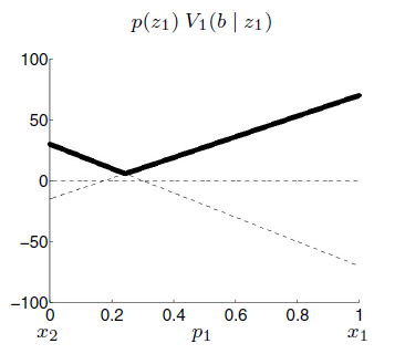
\[\begin{split}p(z_1)v_1(b|z_1)= \max \begin{Bmatrix} -70p_1 & +30(1-p_1) \\ 70p_1 &-15(1-p_1)\\ \end{Bmatrix}\end{split}\]
../../_images/sensing_03.png

  • Same for \(z_2\):

\[\begin{split}p(z_2)v_1(b|z_2)= \max \begin{Bmatrix} -30p_1 & +70(1-p_1) \\ 30p_1 & -35(1-p_1)\\ \end{Bmatrix}\end{split}\]
../../_images/sensing_04.png

So the value function before sensing becomes:

\[\begin{split}\bar{v_1}(b) = \max \begin{Bmatrix} -70p_1 & +30(1-p_1) \\ 70p_1 &-15(1-p_1)\\ \end{Bmatrix} + \max \begin{Bmatrix} -30p_1 & +70(1-p_1) \\ 30p_1 & -35(1-p_1)\\ \end{Bmatrix}\end{split}\]
../../_images/sensing_05.png

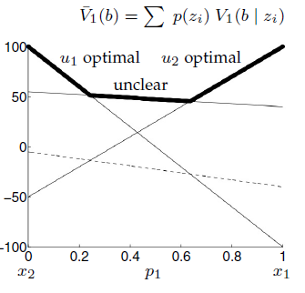
  • However, it seems easier that it is.

  • We actually need to compute the maximum between any sums that adds a linear function from the previous expression.

  • Which leaves us with four possible combination:
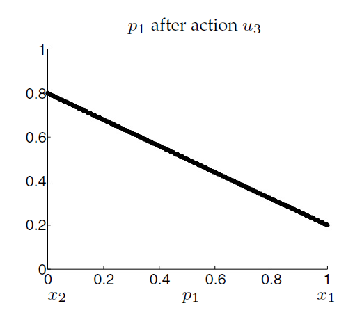
\[\begin{split}\begin{aligned} \bar{v_1}(b) &= \max \begin{Bmatrix} -70p_1 & +30(1-p_1) & -30p_1 & +70(1-p_1) \\ -70p_1 & +30(1-p_1) & +30p_1 & -35(1-p_1)\\ 70p_1 &-15(1-p_1) & -30p_1 & +70(1-p_1)\\ 70p_1 &-15(1-p_1) & +30p_1 & -35(1-p_1) \end{Bmatrix}\\[10pt] &= \max \begin{Bmatrix} -100p_1 & +100(1-p_1) \\ -40p_1 & -5(1-p_1) \\ 40p_1 & +55(1-p_1) \\ 100p_1 & -50(1-p_1) \\ \end{Bmatrix}\\[10pt] &= \max \begin{Bmatrix} -100p_1 & +100(1-p_1) \\ 40p_1 & +55(1-p_1) \\ 100p_1 & -50(1-p_1) \\ \end{Bmatrix}\\ \end{aligned}\end{split}\]

13.1.3. Prediction

  • Now we need to deal with the state transition.

  • Consider we start in \(s_1\) with a probability of \(p_1 = 1\).

    • Then based on our model:

    \[p_1' = p(s_1'|s_2',u_3) = 0.2\]
  • Similarly if \(p_1 = 0\)

    \[p_1' = p(s_1'|s_2',u_3) = 0.8\]
  • And in between the expectations is linear:

\[\begin{split}\begin{aligned} p_1' &= \mathbb{E}\left[ p(s_1'|s,u_3) \right]\\ &= \sum_{i=1}^{N} p(s_1'|s_i,u_3)p_i\\ &= 0.2p_1 + 0.8(1-p_1)\\ &= 0.8-0.6p_1 \end{aligned}\end{split}\]
  • Which give us:

../../_images/predicting_01.png

  • If we project this to our previous value function \(\bar{v_1}(b)\).
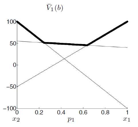
../../_images/predicting_02.png

  • We obtain:

../../_images/predicting_03.png

  • We can see it flattens, because we lose information.

  • Mathematically it’s the projection of \(p_1'\) through \(\bar{v_1}(b)\), giving us:

\[\begin{split}\begin{aligned} \bar{v_1}(b) &= \max \begin{Bmatrix} -100p_1' & +100(1-p_1') \\ 40p_1' & +55(1-p_1') \\ 100p_1' & -50(1-p_1') \\ \end{Bmatrix}\\[10pt] &= \max \begin{Bmatrix} -100(0.8-0.6p_1) & +100(1-(0.8-0.6p_1)) \\ 40(0.8-0.6p_1) & +55(1-(0.8-0.6p_1)) \\ 100(0.8-0.6p_1) & -50(1-(0.8-0.6p_1)) \\ \end{Bmatrix}\\[10pt] &= \max \begin{Bmatrix} -100(0.8-0.6p_1) & +100(0.2+0.6p_1) \\ 40(0.8-0.6p_1) & +55(0.2+0.6p_1) \\ 100(0.8-0.6p_1) & -50(0.2+0.6p_1) \\ \end{Bmatrix}\\[10pt] &= \max \begin{Bmatrix} 60p_1 & -60(1-p_1) \\ 50p_1 & +43(1-p_1) \\ -20p_1 & +70(1-p_1) \\ \end{Bmatrix}\\ \end{aligned}\end{split}\]
  • The value function for step \(T=2\).

  • We just add \(u_1\) and \(u_2\).

\[\begin{split}\bar{v_2}(b) &= \max \begin{Bmatrix} -100p_1 & +100(1-p_1) \\ 100p_1 & -50(1-p_1) \\ 60p_1 & -60(1-p_1) \\ 50p_1 & +43(1-p_1) \\ -20p_1 & +70(1-p_1) \\ \end{Bmatrix}\end{split}\]
  • We remove the uniform cost od \(-1\) from \(u_3\).

\[\begin{split}\bar{v_2}(b) &= \max \begin{Bmatrix} -100p_1 & +100(1-p_1) \\ 100p_1 & -50(1-p_1) \\ 59p_1 & -61(1-p_1) \\ 51p_1 & +42(1-p_1) \\ -21p_1 & +69(1-p_1) \\ \end{Bmatrix}\end{split}\]
../../_images/predicting_05.png

  • We can prune two functions are suboptimal.

\[\begin{split}\bar{v_2}(b) &= \max \begin{Bmatrix} -100p_1 & +100(1-p_1) \\ 100p_1 & -50(1-p_1) \\ 51p_1 & +42(1-p_1) \\ \end{Bmatrix}\end{split}\]

Important

We have done a full backup!