5. Discrete Bayes Filters

We will aply what we have seen before for the localization problem.

5.1. Introduction

Sensors are noisy.

• The GPS in a car reports altitude. Each time it passes the same point in the road it reports a slightly different altitude.

• Kitchen scale gives different readings if we weight the same object twice.

In simple cases the solution is obvious.

• If it gives slightly different readings we can just take a few readings and average them.

• Or replace it with a more accurate sensor.

Example

• If I asked you the heading of my car at this moment you would have no idea.

• You’d proffer a number between \(1^\circ\) and \(360^\circ\) degrees, and have a 1 in 360 chance of being right.

• Now suppose I told you that 2 seconds ago its heading was \(243^\circ\). In 2 seconds my car could not turn very far so you could make a far more accurate prediction.

• You are using past information to more accurately infer information about the present or future.

We discussed the fact that the world is also noisy.

• I may have just braked for a robot or swerved around a pothole.

• Strong winds and ice on the road are external influences on the path of my car.

Important

In robotics literature we call this noise though you may not think of it that way.

5.2. Discrete Bayes Filter

We saw it in the previous topic.

To go further, we will consider that the computer science department has a robot called Alan.

We want to implement a localization algorithm inside it.

A sensor can detect if there is a door or a wall.

It also senses when the robot moves, and reports in which direction the robot has moved.

5.2.1. Problem representation

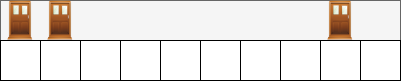
Consider the following problem:

• A hallway with 10 positions

• Numbered from 0 to 9.

• The hallway is circular.

• It’s a global localization problem.

We initialize the belief state as discussed before:

\[b(x_0) = \frac{1}{|X|} = \frac{1}{10}\]

In python:

import numpy as np
belief = np.array([1/10]*10)
print(belief)

[0.1 0.1 0.1 0.1 0.1 0.1 0.1 0.1 0.1 0.1]

Now we can create the map of the hallway. We will use 1 for doors and 0 for walls.

hallway = np.array([1, 1, 0, 0, 0, 0, 0, 0, 1, 0])

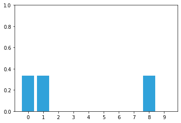
The first data you get from the sensor is door.

• Assume the sensor is perfect.

• From this you conclude that it is in front of a door, but which one?

• We apply the measurement update:

  \[b(x_t) = \eta p(z_t | x_t, m)\bar{b}(x_t)\]

Giving us:

Suppose we were to read the following from Alan’s sensor:

• door

• move right

• door

Activity

Can you deduce Alan’s location?

I designed the hallway layout and sensor readings to give us an exact answer quickly.

5.2.2. Noisy Sensors

Perfect sensors are rare.

Perhaps the sensor would not detect a door if Alan stand in front of it while using a camera, or misread if it is not facing down the hallway.

Thus when you get door you cannot use \(1/3\) as the probability.

You have to assign less than \(1/3\) to each door, and assign a small probability to each blank wall position. Something like:

[.31, .31, .01, .01, .01, .01, .01, .01, .31, .01]

Obviously, we need to do that correctly.

Computation of the likelihood (\(p(z_t|x_t,m)\)) varies per problem.

To make it more general, we will include a parameter in our function that will give the probability that the measurement is correct.

def lh_hallway(hall, z, z_prob):
    """ compute likelihood that a measurement matches
    positions in the hallway."""

    try:
        scale = z_prob / (1. - z_prob)
    except ZeroDivisionError:
        scale = 1e8

    likelihood = np.ones(len(hall))
    likelihood[hall==z] *= scale
    return likelihood

Now that we have a way to calculate the likelihood, we can create the update function:

def normalize(belief):
    return belief / sum(belief)

def update(likelihood, prior):
    return normalize(likelihood * prior)

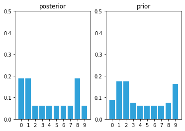
If we test it, with the measurement door with a probability of \(0.75\):

belief = np.array([0.1] * 10)
likelihood = lh_hallway(hallway, z=1, z_prob=.75)
update(likelihood, belief)

array([0.188, 0.188, 0.062, 0.062, 0.062, 0.062, 0.062, 0.062, 0.188, 0.062])

Activity

What happens if we have the measurement door, but with a probability of 0.3?

5.2.3. Incorporating movement

We are able to find an exact solution..

However, that occurred in a world of perfect sensors.

Can we find an exact solution with noisy sensors?

Unfortunately, the answer is no.

Even if the sensor readings perfectly match an extremely complicated hallway map, we cannot be 100% certain that the robot is in a specific position - there is, after all, a tiny possibility that every sensor reading was wrong!

First assume the movement sensor is perfect, and it reports that the robot has moved one space to the right.

Activity

How would it modify our belief array?

def perfect_predict(belief, move):
    """ move the position by `move` spaces, where positive is
    to the right, and negative is to the left
    """
    n = len(belief)
    result = np.zeros(n)
    for i in range(n):
        result[i] = belief[(i-move) % n]
    return result

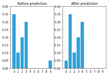
# Initial belief
belief = np.array([.35, .1, .2, .3, 0, 0, 0, 0, 0, .05])

# Belief after update
belief = perfect_predict(belief, 1)

5.2.4. Adding Uncertainty to the Prediction

perfect_predict() assumes perfect measurements, but all sensors have noise.

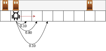
What if the sensor reported that our robot moved one space, but it actually moved two spaces, or zero?

Assume that the sensor’s movement measurement is

• 80% likely to be correct

• 10% likely to overshoot one position to the right

• 10% likely to undershoot one position to the left.

If the robot wants to move 2 cells:

Let’s try coding that:

def predict_move(belief, move, p_under, p_correct, p_over):
    n = len(belief)
    prior = np.zeros(n)
    for i in range(n):
        prior[i] = (
            belief[(i-move) % n]   * p_correct +
            belief[(i-move-1) % n] * p_over +
            belief[(i-move+1) % n] * p_under)
    return prior

If we apply:

belief = [0., 0., 0., 1., 0., 0., 0., 0., 0., 0.]
prior = predict_move(belief, 2, .1, .8, .1)

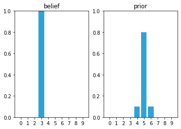
It seems to work, Alan has 10% chance of being in location 4 and 10% in being in location 6.

Warning

It’s a prior, so a prediction! It’s something you can calculate before confirming that the agent has done this action.

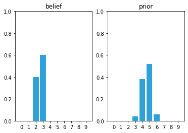
What happens if the initial belief is not 100% certain?

belief = [0, 0, .4, .6, 0, 0, 0, 0, 0, 0]
prior = predict_move(belief, 2, .1, .8, .1)

array([0.  , 0.  , 0.  , 0.04, 0.38, 0.52, 0.06, 0.  , 0.  , 0.  ])

Activity

Try to change the initial belief and movements and see if you can calculate the probabilities manually.

It is important that you understand the calculation behind.

After performing the update the probabilities are not only lowered, but they are scattared across the map.

If the sensor is noisy we lose some information on every prediction.

Important

Suppose we were to perform the prediction an infinite number of times. What would the result be?

If we lose information on every step, we must eventually end up with no information at all, and our probabilities will be equally distributed across the belief array.

Here is an example after 100 iterations.

5.2.5. Generalizing with Convolution

We made the assumption that the movement error is at most one position. But it is possible for the error to be two, three, or more positions.

As programmers we always want to generalize our code so that it works for all cases.

This is easily solved with convolution.

Convolution modifies one function with another function.

In our case we are modifying a probability distribution with the error function of the sensor.

The implementation of predict_move() is a convolution. Formally, convolution is defined as

\[(f \ast g) (t) = \int_0^t \!f(\tau) \, g(t-\tau) \, \mathrm{d}\tau\]

where \(f\ast g\) is the notation for convolving f by g. It does not mean multiply.

Integrals are for continuous functions, but we are using discrete functions. We replace the integral with a summation, and the parenthesis with array brackets.

\[(f \ast g) [t] = \sum\limits_{\tau=0}^t \!f[\tau] \, g[t-\tau]\]

You slide an array called the kernel across another array, multiplying the neighbors of the current cell with the values of the second array.

In our example above we used:

• 0.8 for the probability of moving to the correct location

• 0.1 for undershooting

• 0.1 for overshooting.

We make a kernel of this with the array [0.1, 0.8, 0.1].

All we need to do is write a loop that goes over each element of our array, multiplying by the kernel, and summing the results.

SciPy provides a convolution routine convolve() in the ndimage.filters module. We need to shift the pdf by offset before convolution; np.roll() does that.

The move and predict algorithm can be implemented with one line.

def predict(pdf, offset, kernel, mode='wrap', cval=0.):

    if mode == 'wrap':
        return convolve(np.roll(pdf, offset), kernel, mode='wrap')

    return convolve(shift(pdf, offset, cval=cval), kernel,
                    cval=cval, mode='constant')

5.2.6. Integrating Measurements and Movement updates

Taking back our first example.

hallway = np.array([1, 1, 0, 0, 0, 0, 0, 0, 1, 0])
prior = np.array([.1] * 10)
likelihood = lh_hallway(hallway, z=1, z_prob=.75)
posterior = update(likelihood, prior)

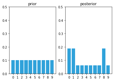
After the first update we have assigned a high probability to each door position, and a low probability to each wall position.

kernel = (.1, .8, .1)
prior = predict(posterior, 1, kernel)

The predict step shifted these probabilities to the right. Now let’s look at what happens at the next sense.

likelihood = lh_hallway(hallway, z=1, z_prob=.75)
posterior = update(likelihood, prior)

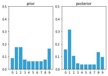
Notice the tall bar at position 1, it increases by detecting another door.

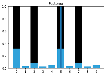
Now we will add an update and then sense the wall.

prior = predict(posterior, 1, kernel)
likelihood = lh_hallway(hallway, z=0, z_prob=.75)
posterior = update(likelihood, prior)

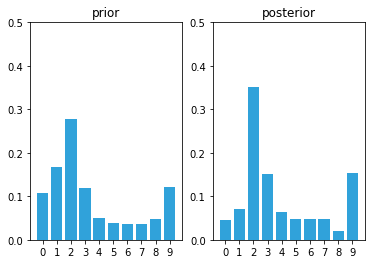
We have a very prominent bar at position 2 with a value of around 35%.

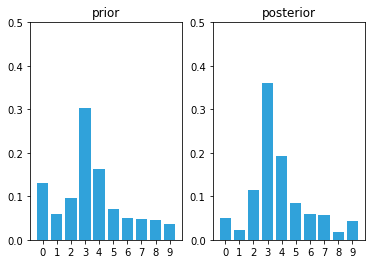
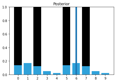
Let’s see one more cycle.

prior = predict(posterior, 1, kernel)
likelihood = lh_hallway(hallway, z=0, z_prob=.75)
posterior = update(likelihood, prior)

5.2.7. The Markov localization Algorithm

Activity

Create a function markov_localization_sim(prior, kernel, measurements, z_prob, hallway) that has parameters:

• prior: The initial prior

• kernel: the kernel

• measurement: a list of measurements

• z_prob: the probability that the measurement is accurate.

• hallway: the hallway

Try it with z_prob=1.

5.2.8. The Effect of Bad Sensor Data

You may be suspicious of the results above because we always passed correct sensor data into the functions.

However, we are claiming that this code implements a filter - it should filter out bad sensor measurements. Does it do that?

To make this easy to program and visualize I will change the layout of the hallway to mostly alternating doors and hallways, and run the algorithm on 6 correct measurements:

hallway = np.array([1, 0, 1, 0, 0]*2)
kernel = (.1, .8, .1)
prior = np.array([.1] * 10)
zs = [1, 0, 1, 0, 0, 1]
z_prob = 0.75
priors, posteriors = markov_localization_sim(prior, kernel, zs, z_prob, hallway)

We have identified the likely cases of having started at position 0 or 5, because we saw this sequence of doors and walls: 1,0,1,0,0.

Now I inject a bad measurement. The next measurement should be 0, but instead we get a 1:

measurements = [1, 0, 1, 0, 0, 1, 1]
priors, posteriors = markov_localization_sim(prior, kernel, measurements, z_prob, hallway)

That one bad measurement has significantly eroded our knowledge.

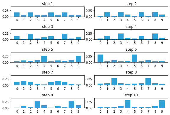
Now let’s continue with a series of correct measurements.

measurements = [1, 0, 1, 0, 0, 1, 1, 1, 0, 0]

5.2.9. Drawbacks and Limitations

Do not be mislead by the simplicity of the examples I chose.

This is a robust and complete filter, and you may use the code in real world solutions. If you need a multimodal, discrete filter, this filter works.

With that said, this filter it is not used often because it has several limitations.

1. The filter does not scale well.

   • Our robot tracking problem used only one variable, \(pos\), to denote the robot’s position.

   • Most interesting problems will want to track several things in a large space. Realistically, at a minimum we would want to track our robot’s \((x,y)\) coordinate, and probably his velocity \((\dot{x},\dot{y})\) as well.

   • We have not covered the multidimensional case, but instead of an array we use a multidimensional grid to store the probabilities at each discrete location.

   • Each update() and predict() step requires updating all values in the grid, so a simple four variable problem would require \(O(n^4)\) running time per time step.

   • Realistic filters can have 10 or more variables to track, leading to exorbitant computation requirements.

2. The filter is discrete, but we live in a continuous world.

   • The histogram requires that you model the output of your filter as a set of discrete points.

   • It gets exponentially worse as we add dimensions. A 100x100 \(m^2\) courtyard requires 100,000,000 bins to get 1cm accuracy.

3. The filter is multimodal.

   • In the last example we ended up with strong beliefs that the robot was in position 4 or 9. This is not always a problem.

   • But imagine if the GPS in your car reported to you that it is 40% sure that you are on D street, and 30% sure you are on Willow Avenue.

4. A forth problem is that it requires a measurement of the change in state.

   • We need a motion sensor to detect how much the robot moves.

Important

It is a good solution for simple problems!