4. Localization

Mobile robot localization is the problem of determining the pose.

It is a critical problem in mobile robotic.

4.1. Different types of localization

In robotics we consider two types of localization:

• Local localization:

  • Position tracking.

  • The initial pose is known.

  • Using filtering techniques

• Global localization:

  • The initial pose is unknown.

  • Find the position in the environment.

The methods to solve these problems are different.

4.2. Markov localization

Markov localization is easy and very similar to the Bayes filter.

The idea is to use the Bayes filter and include map \(m\) of the environment.

Thus the measurement model becomes:

\[p(z_t | x_t, m)\]

We often incorporate the map in the motion model:

\[p(x_t | u_t, x_{t-1}, m)\]

Similarly to the Bayes filter, we use the Markov localization to update and maintain a belief \(b(x_t)\).

Algorithm

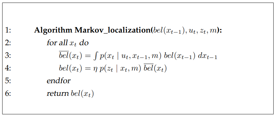
This algorithm works for both localization problem.

4.2.1. Position tracking

We consider that the initial pose is known, thus:

\[\begin{split}b(x_0) = \begin{cases} 1 & \text{if } x_0 = \bar{x}_0\\ 0 & \text{otherwise}\end{cases}\end{split}\]

where \(\bar{x}_0\) is the known initial pose.

It works only a perfect world, in practice we only have an approximation.

Then we use a Gaussian distribution:

\[b(x_0) \sim \mathcal{N} (x_0;\bar{x}_0;\Sigma)\]

where \(\Sigma\) is the covariance of the initial pose uncertainty.

4.2.2. Global localization

In this problem, we don’t know the initial pose.

We assume that the robot can be anywhere with equal probability:

\[b(x_0) = \frac{1}{|X|}\]

where \(|X|\) is the number of states.

4.2.3. Example

Consider the following example.

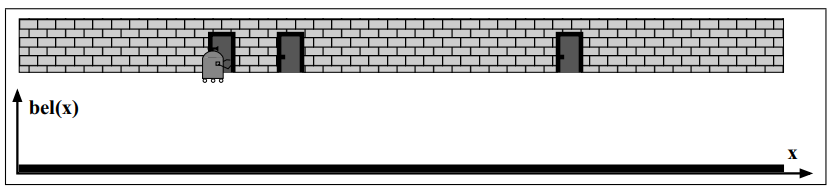
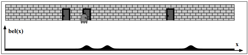
At first the robot doesn’t know where it is.

He only knows the map of the hallway (where the doors are).

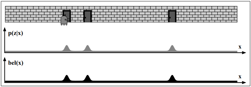
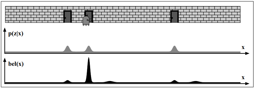
The robot takes a measurement \(z_t\) and apply it to the previous belief \(b(x_t)\).

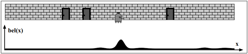
Then it moves and calculate the predicted belief \(\bar{b}(x_t)\).

Because it detects a door (\(z_t\)) it updates the belief \(b(x_t)\).

Then it moves and calculate again the predicted belief \(\bar{b}(x_t)\).