3. Robot Environment Interaction

3.1. Robot environment

Important

A robot is not an isolated system.

• It evolves in an environment, or world, which is a dynamic system.

• The only way for the robot to obtain information about the environment is to use the embedded sensors.

• The sensors will send measurements to the robot.

• The measurements can be noisy.

• Some things cannot be measured by the sensors.

Consequently the robot needs to maintain an internal belief on the state of the environment.

Important

Each interaction of the robot with the environment (using actuators, etc.) can change the environment.

3.2. State

The state characterizes the environment and the robot.

Some variables can have their value change over time, we called them dynamic variables.

• The position of the robot.

• Whereabouts of people in the area.

Some variables are static such as walls.

Important

We denote the state \(x\).

As the state change over time, the state at time \(t\) is denoted \(x_t\).

Activity

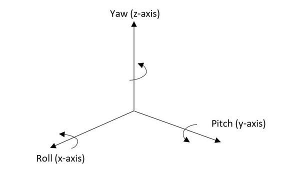
• Consider a 4-wheeled robot in a 3D environment.

• Gives the variables defining the state of a mobile robot evolving in a 3D environment.

• Then, gives a formal definition of the state.

Definition

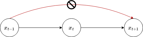
A state \(x_t\) is called complete, if the knowledge of the past states, measurements or controls carry no additional information that would help us predict the future more accurately.

In the previous example, the state we defined is not complete.

We are missing a few things:

1. The robot velocity.

2. The location and features of surrounding objects in the environment.

3. The location and velocities of moving objects and people.

4. Maybe some other variables.

Warning

The definition of completeness does not require the future to be a deterministic function of the state.

The future may be stochastic, but no variables prior to \(x_t\) may influence the stochastic evolution of future states, unless this dependence is mediated through the state \(x_t\).

3.3. Environment Interaction

We can distinguish two types of interaction between a robot and the environment.

1. The robot can influence the state of the environement with its actuators.

2. It can perceive the state with its sensors.

Environment measurement data

The measurement data at time \(t\) will be denoted \(z_t\).

\(z_{t_1:t_2}=z_{t_1}, z_{t_{1+1}}, z_{t_{1+2}}, ..., z_{t_2}\) denotes the set of all measurements acquired from time \(t_1\) to time \(t_2\), for \(t_1 \leq t_2\).

Control data

Control data is denoted \(u_t\). It represents the control action executed by the robot at time \(t\).

\(u_{t_1:t_2}=u_{t_1}, u_{t_{1+1}}, u_{t_{1+2}}, ..., u_{t_2}\) denotes the sequences of control data from time \(t_1\) to time \(t_2\), for \(t_1 \leq t_2\).

When a robot executes a control action \(u_{t-1}\) in the state \(x_{t-1}\) it changes stochastically the state to \(x_{t}\).

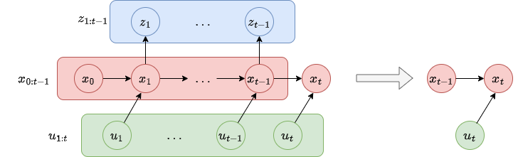
3.4. Probabilistic Generative Laws

If the state change stochastically, then we could calculate the probability of generating \(x_t\):

• We can use all the data accumulated until now: \(u_{1:t-1}, z_{1:t-1}\).

• Then we need to consider all the past states: \(x_{0:t-1}\).

Note

The control and measurement data start at \(t=1\).

It is important to specify that the robot executes first the control action \(u_1\), then takes a measurement \(z_1\).

Activity

• Try to explain why we execute the action first, then measure.

The evolution of state can be given by a probability distribution:

\[p(x_t|x_{0:t-1},z_{1:t-1},u_{1:t})\]

It can be visualize such as:

Example

The problem:

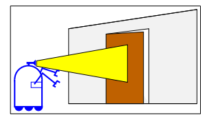
• Suppose a robot that needs to move from one room to another one.

• There is a door that can be either closed or open.

• The robot needs to know if the door is open before trying to move.

Formally:

• We denote the state of the door \(x\).

• We denote \(P(x=\text{open}|z)\) the probability that the door is open.

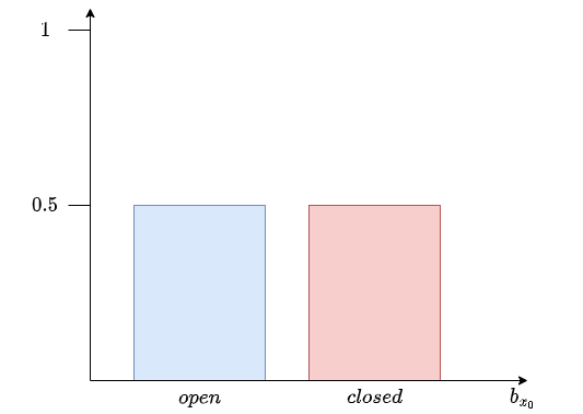
• At time \(t=0\) the robot doesn’t know the state of the door meaning:

  \[p(x_0=\text{open}) = p(x_0=\text{closed}) = 0.5\]

• The robot decides to stay (\(u_1 = \text{stay}\)) and receive a first measurement \(z_1\).

• From experience you know that:

  • \(P(z_1 | x=\text{open}) = 0.6\)

  • \(P(z_1 | x=\text{closed}) = 0.4\)

What is the probability that the door is open?

\[\begin{split}\begin{align} P(x_1=\text{open}|z_1) &= \frac{P(z_1|x_1=\text{open})P(x_0)}{P(z_1)}\\ &= \frac{P(z_1|x_1=\text{open})P(x_0)}{\sum_{x_0'} P(z_1|x_0')P(x_0')}\\ &= \frac{0.6\times 0.5}{0.6\times 0.5 + 0.4\times 0.5}\\ &= 0.6 \end{align}\end{split}\]

• Now, we consider that the robot stay at the same position again (\(u_2 = \text{stay}\) and receive the measurement \(z_2\).

• From experience you know that:

  • \(P(z_2 | x=\text{open}) = 0.5\)

  • \(P(z_2 | x=\text{closed}) = 0.6\)

• The probability that the door is open is:

\[P(x_2=\text{open}|z_2, z_1) = \frac{P(z_2|x_2=\text{open}, z_1)P(x_{0:1}|z_1)}{P(z_2|z_1)}\]

We can see a first issue with this formulation.

• The number of data increase with each time step.

• Increasing the complexity of the probability distribution.

How do we solve this?

If the state \(x\) is complete then \(x_{t-1}\) is a sufficient summary of all previous controls and measurements up to this points (\(u_{1:t-1}, z_{1:t-1}\)).

Concretely, to calculate the probability of \(x_t\), we only need to consider \(u_t\) if we already know \(x_t\).

Meaning,

\[p(x_t|x_{0:t-1},z_{1:t-1},u_{1:t}) = p(x_t|x_{t-1},u_t)\]

If we want to visualize it:

What about measurement?

Again, if \(x_t\) is complete then the probability to measure \(z_t\) is \(p(z_t|x_t)\).

Important

The Markov assumption: \(z_t\) is conditionally independent of \(z_1,...,z_{t-1}\) given \(x\).

\[\begin{split}\begin{split} P(x|z_1,...z_t) &= \frac{P(z_t|x)P(x|z_1,...z_{t-1})}{P(z_t|z_1, ..., z_{t-1})}\\ &= \eta P(z_t|x)P(x|z_1,...z_{t-1})\\ &= \eta_{1..t}\prod_{i=1..t}P(z_i|x)P(x) \end{split}\end{split}\]

Activity

• Come back to the previous example and calculate \(P(x_2=\text{open}|z_2, z_1)\).

• What can you conclude?

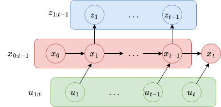
3.4.1. Bayes Network

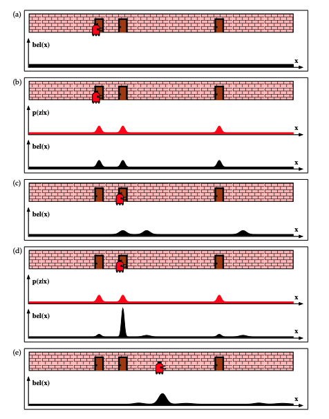
What we discussed before lead us to the dynamic Bayes network.

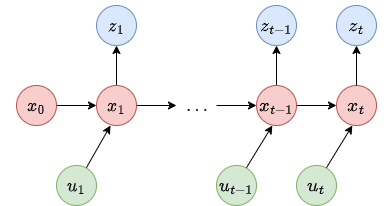
This figure illustrates the evolution of states and measurement through different probabilities.

Note

The state evolve stochastically from time \(t-1\) with \(u_t\) to \(t\). The measurement \(z_t\) is also stochastic.

State transition probability

The state transition probability specifies how the state evolves based on the robot control action \(u_t\).

The probability is given by \(p(x_t|x_{t-1},u_t)\).

Measurement probability

The measurement probability specifies the probabilistic law according to which measurements \(z\) are generated from \(x\).

The probability is given by \(p(z_t|x_t)\), but the probability may not depend of \(t\), then it shall be written \(p(z|x)\).

The measurement can be noisy.

3.4.2. Belief

Another big thing in robotics is the notion of beliefs.

A belief represents the knowledge (or belief) of the robot on the state of the world:

• If you consider a possible state of the robot \(x_t\) corresponding to a position.

• The robot cannot know it’s pose, positions are not measurable directly (even with the GPS).

• The robot will need to infer its position from data (measurement).

We need to distinguish the real state from the internal belief of the robot.

Belief distribution

A belief distribution is posterior probabilities over state variables conditioned on the available data.

The belief over a variable \(x_t\) is denoted \(bel(x_t)\) or \(b(x_t)\).

\[b(x_t) = p(x_t|z_{1:t},u_{1:t})\]

Note

Because a belief represents posterior probabilities we calculate if after the last control action and last measurement received.

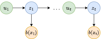
We can different two steps in the belief calculation:

1. The prediction: \(b(x_t) = p(x_t|z_{1:t-1},u_{1:t})\)

2. The correction: Updating \(b(x_t)\) with the measurement \(z_t\).

We can predict the future state using the state transition probability, but as we discuss earlier the control action is not perfect.

So we need to use the measurement to update our prediction.

Important

This distinction is very important!

It means that before executing a control action, you can only calculate the prediction.

3.5. Calculating the belief

To calculate a belief \(b(x_t)\) we are using filters.

3.5.1. Bayes filter

The most general one is the Bayes filter algorithm:

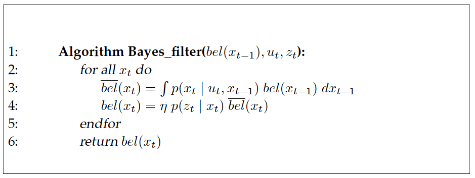
It is a general filter, because it applies the belief formula as previously defined.

• The filter takes three parameters:

  • The belief at step \(t-1\)

  • The action control \(u_t\)

  • The measurement received \(z_t\).

• The algorithm starts by predicting the new state using the control action (line 3), so the prediction.

• Then update (or correct) the prediction using the measurement, so the correction.

3.5.2. Application

Let’s try to use the filter on the previous example.

We have a robot in front of a door that can be ever closed or open and the robot has two control actions available either doing nothing or push the door.

At the time step \(t=0\) the robot doesn’t know if the door is open or closed, so it gives us:

\[\begin{split}\begin{align} b(x_0 = \text{open}) &= 0.5\\ b(x_0 = \text{closed}) &= 0.5\\ \end{align}\end{split}\]

We are defining the state transition probabilities as:

State \(t\)	Control action	State \(t-1\)	Probability
\(x_{t} = \text{open}\)	\(u_{t} = \text{push}\)	\(x_{t-1} = \text{open}\)	1
\(x_{t} = \text{closed}\)	\(u_{t} = \text{push}\)	\(x_{t-1} = \text{open}\)	0
\(x_{t} = \text{open}\)	\(u_{t} = \text{push}\)	\(x_{t-1} = \text{closed}\)	0.8
\(x_{t} = \text{closed}\)	\(u_{t} = \text{push}\)	\(x_{t-1} = \text{closed}\)	0.2
\(x_{t} = \text{open}\)	\(u_{t} = \text{nothing}\)	\(x_{t-1} = \text{open}\)	1
\(x_{t} = \text{closed}\)	\(u_{t} = \text{nothing}\)	\(x_{t-1} = \text{open}\)	0
\(x_{t} = \text{open}\)	\(u_{t} = \text{nothing}\)	\(x_{t-1} = \text{closed}\)	0
\(x_{t} = \text{closed}\)	\(u_{t} = \text{nothing}\)	\(x_{t-1} = \text{closed}\)	1

We also need to define measurement probabilities:

Measurement \(t\)	State \(t\)	Probability
\(z_{t} = \text{open}\)	\(x_{t} = \text{open}\)	0.6
\(z_{t} = \text{closed}\)	\(x_{t} = \text{open}\)	0.4
\(z_{t} = \text{open}\)	\(x_{t} = \text{closed}\)	0.2
\(z_{t} = \text{closed}\)	\(x_{t} = \text{closed}\)	0.8

Note

The state transition and measurement probabilities depend of the problem and can either be calculated or are given by experts.

Example

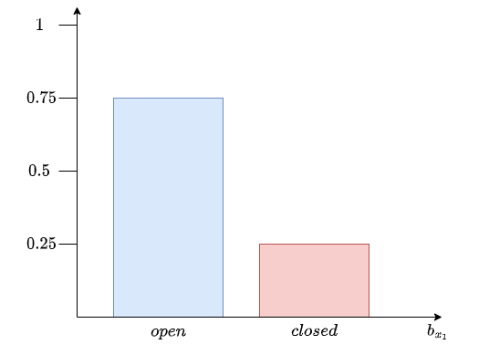
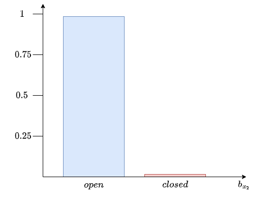
Suppose we have the following sequence: \(u_{1} = \text{nothing}, z_1 = \text{open}, u_{2} = \text{push}, z_2 = \text{open}\).

If we use the Bayes filter to calculate \(b(X_1)\):

\[\begin{split}\begin{split} \bar{b}(x_1) &= \int p(x_1|u_1,x_0)b(x_0)dx_0\\ &=\sum_{x_0}p(x_1|u_1,x_0)b(x_0)\\ &=p(x_1|u_1=\text{nothing},x_0=\text{open})b(x_0=\text{open}) + p(x_1|u_1=\text{nothing},x_0=\text{closed})b(x_0=\text{closed})\\ \end{split}\end{split}\]

We can calculate for each state possible:

\[\begin{split}\begin{split} \bar{b}(x_1=\text{open}) &= p(x_1=\text{open}|u_1=\text{nothing},x_0=\text{open})b(x_0=\text{open})\\ &+ p(x_1=\text{open}|u_1=\text{nothing},x_0=\text{closed})b(x_0=\text{closed})\\ &= 1\times 0.5 + 0\times 0.5\\ &= 0.5 \end{split}\end{split}\]

\[\begin{split}\begin{split} \bar{b}(x_1=\text{closed}) &= p(x_1=\text{closed}|u_1=\text{nothing},x_0=\text{open})b(x_0=\text{open})\\ &+ p(x_1=\text{closed}|u_1=\text{nothing},x_0=\text{closed})b(x_0=\text{closed})\\ &= 0\times 0.5 + 1\times 0.5\\ &= 0.5 \end{split}\end{split}\]

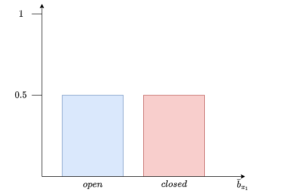
Now, we can use the measurement to correct the predictions:

\[b(x_1) = \eta p(z_1 = \text{open}|x_1)*\bar{b}(x_1)\]

For each state:

\[ \begin{align}\begin{aligned}\begin{split}\begin{split} b(x_1=\text{open}) &= \eta p(z_1 = \text{open}|x_1 = \text{open})*\bar{b}(x_1 = \text{open})\\ &= \eta 0.6\times0.5\\ &= \eta 0.3 \end{split}\end{split}\\\begin{split}\begin{split} b(x_1=\text{closed}) &= \eta p(z_1 = \text{open}|x_1 = \text{closed})*\bar{b}(x_1 = \text{closed})\\ &= \eta 0.2\times0.5\\ &= \eta 0.1 \end{split}\end{split}\end{aligned}\end{align} \]

Now we can calculate \(\eta\):

\[\eta = (0.3+0.1)^{-1} = 2.5\]

So we have:

\[\begin{split}\begin{split} b(x_1=\text{open}) &= 0.75\\ b(x_1=\text{closed}) &= 0.25\\ \end{split}\end{split}\]

Now, we are repeating the process.

\[\begin{split}\begin{split} \bar{b}(x_2) &= \int p(x_2|u_2,x_1)b(x_1)dx_1\\ &=\sum_{x_1}p(x_2|u_2,x_1)b(x_1)\\ &=p(x_2|u_2=\text{push},x_1=\text{open})b(x_1=\text{open}) + p(x_2|u_2=\text{push},x_1=\text{closed})b(x_1=\text{closed})\\ \end{split}\end{split}\]

We calculate the prediction at time \(t=2\) for each state possible:

\[\begin{split}\begin{split} \bar{b}(x_2=\text{open}) &= p(x_2=\text{open}|u_2=\text{push},x_1=\text{open})b(x_1=\text{open})\\ &+ p(x_2=\text{open}|u_2=\text{push},x_1=\text{closed})b(x_1=\text{closed})\\ &= 1\times 0.75 + 0.8\times 0.25\\ &= 0.95 \end{split}\end{split}\]

\[\begin{split}\begin{split} \bar{b}(x_2=\text{closed}) &= p(x_2=\text{closed}|u_2=\text{push},x_1=\text{open})b(x_1=\text{open})\\ &+ p(x_2=\text{closed}|u_2=\text{push},x_1=\text{closed})b(x_1=\text{closed})\\ &= 0\times 0.75 + 0.2\times 0.25\\ &= 0.05 \end{split}\end{split}\]

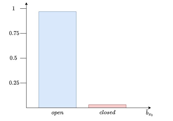
Then, we correct:

\[b(x_2) = \eta p(z_2 = \text{open}|x_2)*\bar{b}(x_2)\]

For each state:

\[ \begin{align}\begin{aligned}\begin{split}\begin{split} b(x_2=\text{open}) &= \eta p(z_2 = \text{open}|x_2 = \text{open})*\bar{b}(x_2 = \text{open})\\ &= \eta 0.6\times 0.95\\ &= \eta 0.57 \end{split}\end{split}\\\begin{split}\begin{split} b(x_2=\text{closed}) &= \eta p(z_2 = \text{open}|x_2 = \text{closed})*\bar{b}(x_2 = \text{closed})\\ &= \eta 0.2\times 0.05\\ &= \eta 0.01 \end{split}\end{split}\end{aligned}\end{align} \]

Now we can calculate \(\eta\):

\[\eta = (0.57+0.01)^{-1} = 1.72\]

So we have:

\[\begin{split}\begin{split} b(x_2=\text{open}) &= 0.98\\ b(x_2=\text{closed}) &= 0.02\\ \end{split}\end{split}\]

Activity

1. Implement the Bayes filter in python.

2. Generate randomly different sequences of control action, and measurement for the previous problem over \(t=1..10\) steps.

3. Use the filter to calculate the belief at each time step \(t\). You should start with \(b(x_0 = \text{open}) = b(x_0 = \text{closed}) = 0.5\).

4. Plot the evolution of the probability for each state.

3.5.3. Not as simple as it seems

We need to talk about the belief representation.

We used the Bayes filter on a problem with discrete states. Generally, it’s not the case for real-life applications.

• Implies that for continuous states, we have an integral in the calculation.

• Usually, we need to approximate the belief state.

• Thus the Bayes filter cannot be applied easily.

When approximating a belief, we need to keep some things in mind:

• Computational efficiency.

• Accuracy of the approximation.

• Ease of implementations.