7. Sensor Models
We have covered a lot of things until now, but we are missing one thing.
We need to cover the sensors, because we assumed that we received measurements without defining how it is done.
Important
The objective is to determine \(p(z|x)\).
The probability to receive a specific measurement in a state \(x\).
Robots can have lots of different sensors:
Contact sensors: Bumpers
Internal sensors:
Accelerometers
Gyroscopes
Compasses
Proximity sensors:
Sonar
Radar
Laser
Infrared
Visual sensors: Cameras
Satellite-based sensors: GPS
A very common type of sensor for indoor robots is proximity sensors.
Most of them are called beam-based sensors (sonar, laser, etc.).
7.1. Beam-Based Sensor Model
A sensor does not perceive only one measurement.
Like a camera does not receive only one measurement (brightness, saturation, color).
Consider a measurement \(z_t\) at time \(t\).
It can take \(K\) different values:
where \(z^k_t\) is an individual measurement.
We will consider that individual measurement are independent.
where \(m\) represents the map.
Warning
It is an ideal case, individual measurements are not always independent.
Beam-Based model incorporates four types of measurement errors:
small measurement noise
unexpected objects
failures to detect objects
unexplained random noise
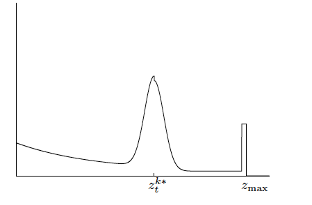
7.1.1. Correct range
Let us define \(z^{k*}_t\) the true range of the object measured by \(z^k_t\).
However, the value returned by the sensors is subject to error.
The measurement noise is modelled by a Gaussian \(\mathcal{N}(z_t^{k*}, \sigma^2_{\text{hit}})\).
The following figure illustrates the Gaussian:
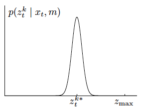
So, to calculate the probability \(p_{\text{hit}}(z_t^k|x_t, m)\) we use the univariate normal distribution formula:
where \(\eta\) is a normalizer:
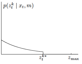
7.1.2. Unexpected Object
In robotics the environment is rarely static, so objects not contained in the map can be appearing.
Pedestriant on a road.
Birds with UAVs
etc.
The range \(z_t^k\) can be shorter than \(z_t^{k*}\).
If you think about it an unexpected obstacle is more likely to be closer than further away.
Mathematically, the probability is described as an exponential distribution of parameters \(\lambda_{\text{short}}\).
So we can calculate the probability \(p_{short}(z^k_t| x_t, m)\) as:
where \(\eta = \frac{1}{1-e^{-\lambda_{\text{short}}z_t^{k*}}}\).
This probability function is illustrated below:
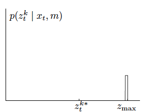
7.1.3. Failures
Sometimes obstacles are missed.
It can happen with lasers when sensing black objects, with GPS if you go in a tunnel.
When it happens, usually sensors are sending a max-range measurement.
It’s quite frequent, so we cannot skip it.
We model this case with a point-mass distribution centered at \(z_\text{max}\):
Even if it’s not really a probability distribution, we draw it like it is:
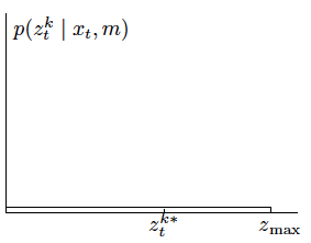
7.1.4. Random Measurements
These sensors can produce unexplainable measurements.
It’s very hard to explain these readings, so we model them with a uniform distribution:
If we plot this distribution, we obtain:
7.1.5. Putting Everything Together
We finally mix the four different distributions by a weighted average defined by the parameters:
\(z_{\text{hit}}\)
\(z_{\text{short}}\)
\(z_{\text{max}}\)
\(z_{\text{rand}}\)
These parameters summing to \(1\).
The probability of the measurement becomes:
It will create a new density function:
Activity
Implement the following function that calculates the individual probabilities:
def p_hit(z_meas, z_true, sigma, z_max):
    pass

def p_short(z_meas, z_true, l_short):
    pass

def p_max(z_meas, z_max):
    pass
Use the previous functions to implement the last function that put everything together:
#  z_weight is a vector containing the weights for each probability
def prob(z_meas, z_true, z_max, z_weight, sigma, l_short):
    pass
Example
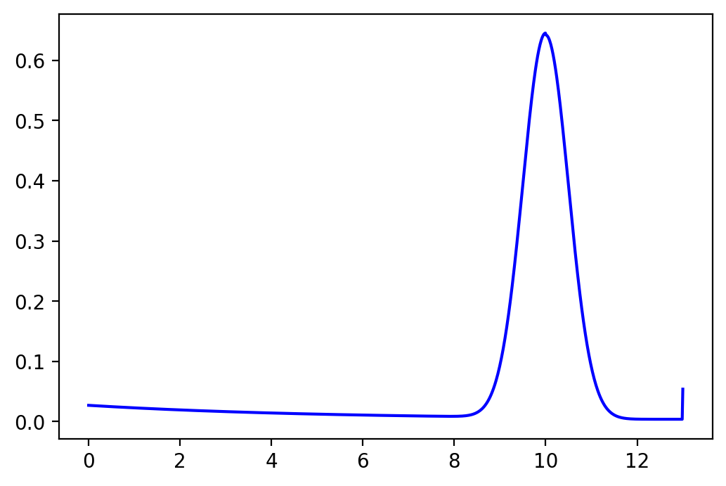
We can test the previous functions.
The robot is not moving and has one beam sensor.
Consider the following properties for the beam sensor:
A distance maximal \(z_{\text{max}}\) of 13 meters.
A parameter \(\lambda_{\text{short}}\) of \(0.2\).
Consider the vector of weights \(\left[0.8, 0.1, 0.05, 0.05 \right]\).
Finally, the true measurement \(z^{k^*}\) is 10 meters.
We can implement it in python:
z_meas = np.linspace(0, 13, 1000)
z_true = 10
z_max = 13
sigma = 0.5
l_short = 0.2
z_weights = [0.8, 0.1, 0.05, 0.05]
probs = []
for z in z_meas:
probs.append(prob(z, z_true, z_max, z_weights, sigma, l_short))
fig, ax = plt.subplots(1, 1)
ax.plot(z_meas, probs,'b-')
plt.show()
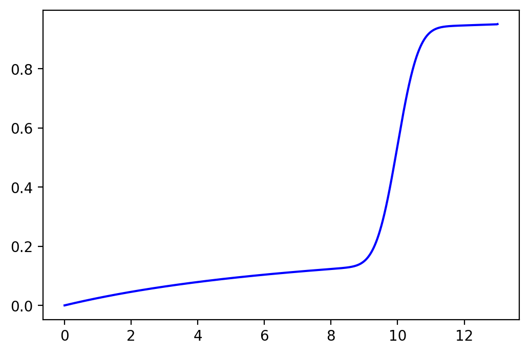
cdf = np.cumsum(probs)*(z_meas[1]-z_meas[0])
fig, ax = plt.subplots(1, 1)
ax.plot(z_meas, cdf,'b-')
plt.show()
It plots the probability distribution;
It also plot the CDF to be sure that it sums to 1:
7.1.6. Using every sensors
Now that we are able to calculate the probability for one sensor, we can calculate the total probability \(p(z_t|x_t, m)\).
The function is quite simple:
Initialize the probability \(p\) to 1.
For each sensor:
Compute the probability \(q\)
Multiply \(q\) with \(p\).
Return \(p\)
7.1.7. Adjusting the Intrinsic Model Parameters
All the parameters we talked about, need to be calculated.
There are two ways to do it:
You adjust the parameters manually to match the measurement of the sensor.
You learn them with an algorithm.
These methods are outside the scope of the course.
7.1.8. Limitations
The Beam-based model is:
not smooth for small obstacles and at edges.
not very efficient.
7.2. Featured-Based Models
The beam-based models are based on raw sensor measurement.
Another very popular approach is to extract features from the measurements.
We can consider a feature extractor \(f\), then the features extracted are given by \(f(z_t)\).
Important
In this course we will not discuss how we can extract the features from an environment.
A very common application is landmark measurements.
Landmarks are just a word that represents any distinct objects.
Activity
Think about possible landmark for autonomous vehicles.
For wheeled robots in a building?
7.2.1. Landmark Measurements
Usually we denote a feature \(f_t^n\) as:
where \(r^i_t\) is the range, \(\phi^i_t\) is the heading and \(s_t^i\) is the signature.
Basically, it’s the measurement you receive from the sensor.
The measurement without noise is just standard geometric calculation.
We will model the noise as Gaussian white noises, the noises are independent for each variable.
Concretely for each landmark \(j \in m\):
where \(\epsilon_{\sigma^2_r}, \epsilon_{\sigma^2_\phi}, \epsilon_{\sigma^2_s}\) are zero-mean Gaussian error variables with standard deviation \(\sigma_r, \sigma_\phi, \sigma_s\).
7.2.2. Calculating Likelihood of Landemark
It is now, very easy to calculate the likelihood of a feature to be a specific landmark \(m_j\):
Calculate \(\hat r = \sqrt{(m_{j,x}-x)^2 + (m_{j,y}-y)^2}\)
Calculate \(\hat \phi = \text{atan2} (m_{j,y}-y, m_{j,x}-x)\)
Calculate the probability \(p = \text{prob}(r^i_t - \hat r, \sigma_r)\times \text{prob}(\phi^i_t - \hat \phi, \sigma_\phi) \times \text{prob}(s^i_t - \hat s, \sigma_s)\)
\(\text{prob}(\cdot,\cdot)\) is the pdf of a Gaussian of standard deviation \(\sigma\).
Activity
Implement the function that calculates the likelihood of a measurement.
Do not consider the signature.
Now consider the small following problem:
You try to locate your friend using his cell phone signal.
The two cell towers are in \((12,4)\) and \((5,7)\).
The two possible position of your friends are his house \((6,3)\) and StFX \((10,8)\).
You receive the following signals:
From the first tower \(r = 3.9\) and \(\sigma_1 = 1\).
From the second tower \(r = 4.5\) and \(\sigma_2 = \sqrt{1.5}\).
Calculate the probability of your friend being at home and at the university.