8. Grid Localization

The Markov localization doesn’t consider raw measurement.

The grid localization algorithm can solve global localization problem using raw measurement.

The algorithm uses a histogram filter:

• Take a continuous environment.

• Discretize it in many regions.

• Calculate the belief for each region.

8.1. The Algorithm

The algorithm is similar to the Bayes filter:

• We want to maintain a belief \(b(x_t)\).

• As we use a grid \(b(x_t)= \{p_{k,t}\}\).

  where \(p_{k,t}\) is the probability over a cell \(\mathbf{x}_k\).

• All legitimate poses forms a partition of the space:

  \(\text{domain}(X_t) = \mathbf{x}_{1,t} \cup \mathbf{x}_{2,t} \cup \dots \cup \mathbf{x}_{K,t}\)

The figure below illustrates how we can create a domain of all poses possible:

Note

Usually, we choose a granularity of 15 cm for the \(x\) and \(y\) dimension and \(5\) degrees for the rotational dimension.

The pseudocode of the algorithm is:

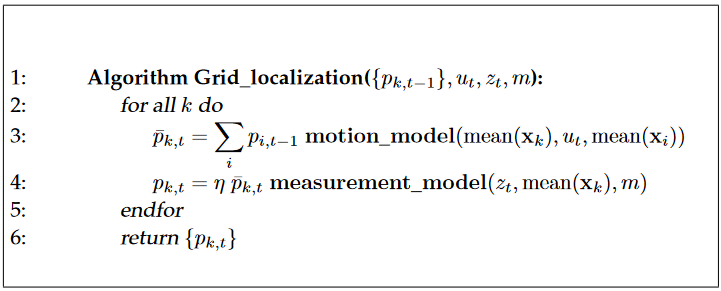
The algorithm takes four parameters:

• The current belief \(b(x_t) = \{p_{k,t}\}\).

• The control action \(u_t\).

• The measurement \(z_t\).

• The map.

The prediction is done with the motion model of the robot, that we covered in a previous topic.

The prediction is updated using the measurement model seen previously.

Important

The \(\text{mean}(\mathbf{x}_k)\) is the center of a grid cell \(\mathbf{x}_k\).

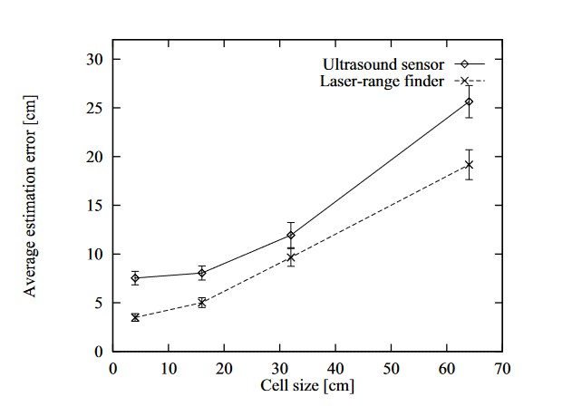
8.2. Grid resolutions

A key in grid localization is the resolution of the grid.

It impacts:

• The type of sensor model we can use.

• The way the belief is calculated.

• The type of results we can expect.

A common representation is the metric representation:

• The state space is divided into fine-grained cells of uniform sized.

• Like mentioned before 15 cm is the norm.

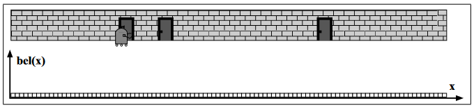
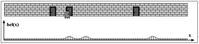
If we take a previous example with the robot in a hallway, we can divide the hallway in small cells:

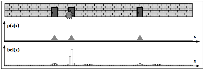
We receive a measurement \(z_t\) that we use to update the belief:

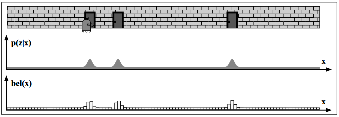
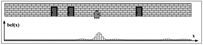
Then the robot is executing an action, which leads to a new predicted belief:

Then, it receives a new measurement:

And it continues:

Note

High-resolution sensor needs some particular process, as the \(p(z_t|x_t)\) may vary drastically inside each cell \(\mathbf{x}_{k,t}\).