9. Monte-Carlo Localization
Another popular localization method is Monte-Carlo localization.
The main difference grid localization is that, this method doesn’t require to discretize the environment.
9.1. The idea
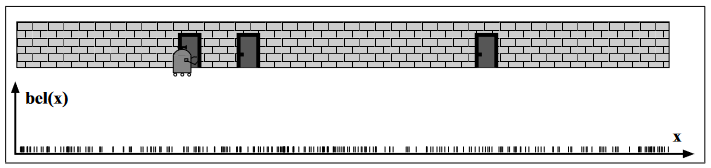
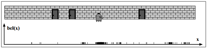
To illustrate the idea,we will consider the hallway example.
With MC localization we create our initial belief by sampling a set of pose particles randomly and uniformly:
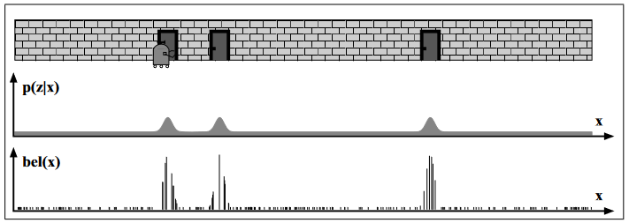
When the robot receives a measurement, it calculates the probability of this measurement for each particle.
Then it applies it to the current set of particles modifying their weights:
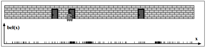
Then the robots apply a control action.
A new particle set is resampled following the robot motion model and the current particle set and weight.
The robot sense again and update the new particle set:
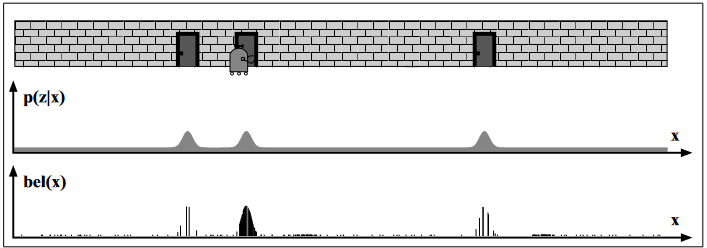
And we repeat:
9.2. The Algorithm
The pseudocode of the algorithm is:
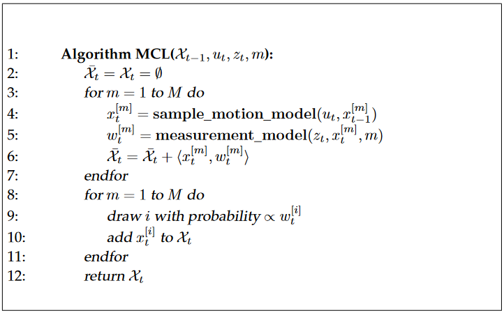
The belief \(b(x_t)\) is represented by a set of \(M\) particles:
For each sample we calculate the predicted particles using the motion model (line 4).
Then we calculate the weight of the particle using the measurement and measurement model (line 5).
After that we resample to obtain the new belief:
It sample a particule based on the weight of each particle.
Add this particle to the new set of particles.
Activity
Implement the algorithm in python.
Test it with the motion and measurement model of your choice.
9.3. Properties of MC localization
MC localization can approximate almost any distribution.
Increasing the number of particles increases the accuracy, but increase the computational resources needed.
Finally, this algorithm cannot recover from a critical failure or if the robot is displaced manually.